BiocAlphaMissense: Bioconductor interfaces to AlphaMissense pathogenicity findings
Vincent J. Carey, stvjc at channing.harvard.edu
September 24, 2023
Source:vignettes/BiocAlphaMissense.Rmd
BiocAlphaMissense.RmdIntroduction
AlphaMissense (Science 2023) is a machine learning procedure for inferring pathogenicity of single nucleotide substitutions in the human proteome. Text files are distributed by the authors, and these have been tabix-indexed for use in this package. Note that the pathogenicity data are produced under a license that forbids commercial use.
The package described here can currently be installed using
BiocManager::install("vjcitn/BiocAlphaMissense")Gene level summaries; binding to EnsDb annotations
Production of annotated gene level summaries
We retrieved the gene level summary data on 24 Sept 2023, e.g., the hg38 file. This was transformed to a data.frame instance and lodged in the package for use via data(am_genemns_hg38). The annotation used at the source is GENCODE. An additional column, tx_id, is added, which removes the GENCODE version qualifiers (.n[n]$). This simplifies merging with EnsDb gene and transcript annotation.
Let’s bind the average pathogenicity scores to our transcript annotation.
library(BiocAlphaMissense)
library(EnsDb.Hsapiens.v79)
tx38 = transcripts(EnsDb.Hsapiens.v79)
tx38df = as.data.frame(tx38)
data(am_genemns_hg38)
tx38df = merge(tx38df, am_genemns_hg38, by="tx_id")
Note that there are 19233 scores available in the gene-level summary.
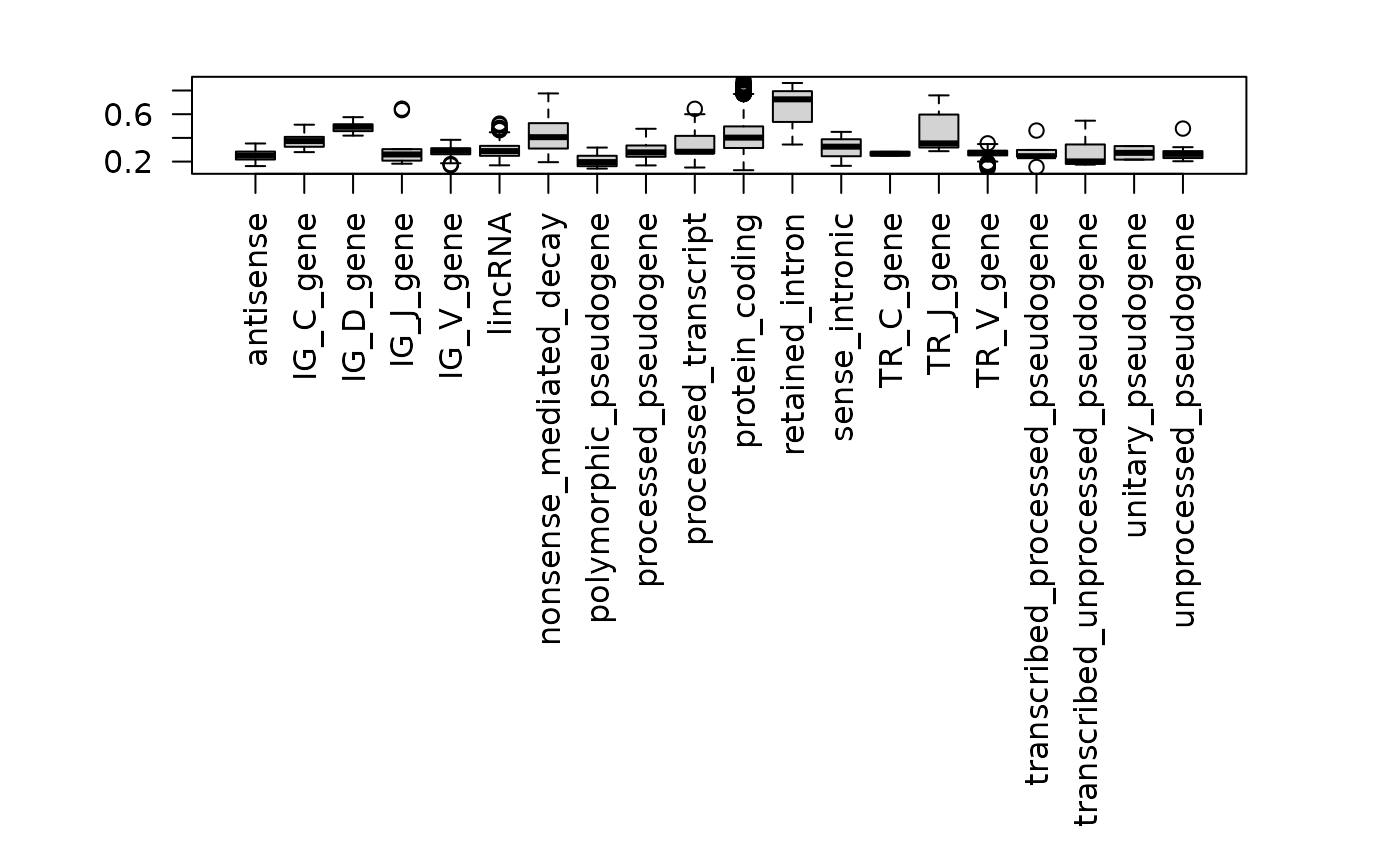
Pathogenicity across annotated biotypes
As a simple sanity check, we check distributions of pathogenicity scores across transcript biotype.
What are the gene level averages?
In this section we pick a gene and look at the landscape of pathogenicity scores to see what the averaging process is doing.
First, get gene address for ORDML3.
gg = genes(EnsDb.Hsapiens.v79)
gdf = as(gg, "data.frame")
tx38df2= merge(tx38df, gdf[,c("gene_id", "symbol")], by="gene_id")
myp = gg[gg$symbol=="ORMDL3"]
Now get the SNV-level data in this region.
amis_txf = get_alphamis_txf(build="hg38")
library(Rsamtools)
seqlevelsStyle(myp) = "UCSC"
## Warning in (function (seqlevels, genome, new_style) : cannot switch some
## GRCh38's seqlevels from NCBI to UCSC style
sc = read.delim(text=scanTabix(amis_txf, param=myp)[[1]], h=FALSE)Plot the scores against the genomic coordinate.
plot(sc$V2, sc$V9,xlab="bp chr17", ylab="substitution-specific pathogenicity")
Check the average score from the SVN-level data against the reported mean.
mean(sc$V9) # SNV## [1] 0.6466165
tx38df2[tx38df2$symbol=="ORMDL3",] # reported mean pathogenicity## gene_id tx_id seqnames start end width strand
## 12511 ENSG00000172057 ENST00000394169 17 39922277 39926841 4565 -
## tx_biotype tx_cds_seq_start tx_cds_seq_end tx_name
## 12511 protein_coding 39922550 39924203 ENST00000394169
## transcript_id mean_am_pathogenicity symbol
## 12511 ENST00000394169.5 0.6466168 ORMDL3A quick look at single-nucleotide data
The following code draws the first 10 records and places them in a data.frame. Note that 600 MB of bgzipped text and a tabix index will be retrieved and cached on first attempt.
library(BiocAlphaMissense)
library(Rsamtools)
amis_txf = get_alphamis_txf(build="hg38")
amis_txf
## class: TabixFile
## path: /home/vincent/.cache/R/BiocFileC.../a86b4ba7d3c4_AlphaMissense_hg38.tsv.gz
## index: /home/vincent/.cache/R/Bioc.../a86b74da37cb_AlphaMissense_hg38.tsv.gz.tbi
## isOpen: FALSE
## yieldSize: NA
yieldSize(amis_txf) = 10L
df10 = read.delim(text=scanTabix(amis_txf)[[1]], h=FALSE)
data(amnames)
names(df10) = amnames
df10
## CHROM POS REF ALT genome uniprot_id transcript_id protein_variant
## 1 chr1 69094 G T hg38 Q8NH21 ENST00000335137.4 V2L
## 2 chr1 69094 G C hg38 Q8NH21 ENST00000335137.4 V2L
## 3 chr1 69094 G A hg38 Q8NH21 ENST00000335137.4 V2M
## 4 chr1 69095 T C hg38 Q8NH21 ENST00000335137.4 V2A
## 5 chr1 69095 T A hg38 Q8NH21 ENST00000335137.4 V2E
## 6 chr1 69095 T G hg38 Q8NH21 ENST00000335137.4 V2G
## 7 chr1 69097 A G hg38 Q8NH21 ENST00000335137.4 T3A
## 8 chr1 69097 A C hg38 Q8NH21 ENST00000335137.4 T3P
## 9 chr1 69097 A T hg38 Q8NH21 ENST00000335137.4 T3S
## 10 chr1 69098 C A hg38 Q8NH21 ENST00000335137.4 T3N
## am_pathogenicity am_class
## 1 0.2937 likely_benign
## 2 0.2937 likely_benign
## 3 0.3296 likely_benign
## 4 0.2609 likely_benign
## 5 0.2922 likely_benign
## 6 0.2030 likely_benign
## 7 0.0929 likely_benign
## 8 0.1264 likely_benign
## 9 0.0979 likely_benign
## 10 0.1121 likely_benignChecking against GWAS hits: asthma example
We used the EBI GWAS catalog and searched for “sthma” in the MAPPED_TRAIT field. The resulting records are in a GRanges instance, accessible via data(amentgr).
## [1] 3488
amentgr[1:3,c("STRONGEST.SNP.RISK.ALLELE", "PUBMEDID")]## GRanges object with 3 ranges and 2 metadata columns:
## seqnames ranges strand | STRONGEST.SNP.RISK.ALLELE PUBMEDID
## <Rle> <IRanges> <Rle> | <character> <numeric>
## [1] 17 39909987 * | rs2290400-C 27439200
## [2] 2 15780199 * | rs2544523-T 24993907
## [3] 5 116261351 * | rs10043228-T 24993907
## -------
## seqinfo: 23 sequences from GRCh38 genome; no seqlengthsThe coincidence of these GWAS hits with AlphaMissense results (amis_txf created above) can be computed quickly,.
library(Rsamtools)
library(GenomeInfoDb)
seqlevels(amentgr) = paste0("chr", seqlevels(amentgr)) # if off line
yieldSize(amis_txf) = NA_integer_
lk = scanTabix(amis_txf, param=amentgr)
Some of the positions with GWAS hits don’t correspond to results from AlphaMissense. These positions are empty components of the list returned by scanTabx. They are removed and the scanTabix results are converted to a data.frame.
ok = which(vapply(lk, function(x)length(x)>0, logical(1)))
cc = c("character", "character", "character", "character", "character",
"character", "character", "character", "numeric", "character")
intsect = lapply(lk[ok],
   function(x) read.delim(text=x, h=FALSE, colClasses=cc))
intsect_df = do.call(rbind, intsect)
data(amnames)
names(intsect_df) = amnames
head(intsect_df,3)
## CHROM POS REF ALT genome uniprot_id
## chr4:38798089-38798089.1 chr4 38798089 T A hg38 Q15399
## chr4:38798089-38798089.2 chr4 38798089 T C hg38 Q15399
## chr4:38798089-38798089.3 chr4 38798089 T G hg38 Q15399
## transcript_id protein_variant am_pathogenicity
## chr4:38798089-38798089.1 ENST00000502213.6 N248I 0.1326
## chr4:38798089-38798089.2 ENST00000502213.6 N248S 0.0737
## chr4:38798089-38798089.3 ENST00000502213.6 N248T 0.1079
## am_class
## chr4:38798089-38798089.1 likely_benign
## chr4:38798089-38798089.2 likely_benign
## chr4:38798089-38798089.3 likely_benignAt this point, intsect_df is the collection of all substitution scores at asthma GWAS hits. We focus on the substitutions reported as risk alleles.
amentgr$RISK_ALLELE = gsub("(.*-)", "", amentgr$STRONGEST.SNP.RISK.ALLELE)To join the missense classes with the coincident GWAS hits we build a “key” for each table and then join.
intsect_df$key = with(intsect_df, paste(CHROM, POS, ALT, sep=":"))
ament_df = as.data.frame(amentgr)
ament_df$key = with(ament_df, paste(seqnames, CHR_POS, RISK_ALLELE, sep=":"))
ia = dplyr::inner_join(intsect_df, ament_df, by="key", relationship = "many-to-many")
iau = ia[!duplicated(ia$key),]
table(iau$am_class)
##
## ambiguous likely_benign likely_pathogenic
## 1 15 3Some of the information about the likely pathogenic substitutions that have been identified as hits for asthma is collected here:
iau |>
  dplyr::filter(am_class == "likely_pathogenic") |>
  dplyr::select(CHR_ID, CHR_POS, STRONGEST.SNP.RISK.ALLELE,
  OR.or.BETA, MAPPED_TRAIT, MAPPED_GENE, am_class)
## CHR_ID CHR_POS STRONGEST.SNP.RISK.ALLELE OR.or.BETA MAPPED_TRAIT
## 1 5 14610200 rs16903574-G 1.0862118 asthma
## 2 1 12115601 rs2230624-A 0.1618169 asthma
## 3 9 128721272 rs11539209-A NA asthma
## MAPPED_GENE am_class
## 1 OTULINL likely_pathogenic
## 2 TNFRSF8 likely_pathogenic
## 3 ZDHHC12 likely_pathogenic