A: Labelling PBMCs using Human Primary Cell Atlas
Vincent J. Carey, stvjc at channing.harvard.edu
May 16, 2023
A_SingleR.RmdIntroduction
This vignette provides a very brief introduction to the use of Bioconductor packages and functions to work with single cell RNA-seq data. The tasks include
- learning about SummarizedExperiment to manage multiple samples constituting reference expression data on selected cell types
- learning about SingleCellExperiment to work with expression patterns on thousands of cells
- using the SingleR package and function to train a classifier of cell types and label a sample of PBMCs assayed with TENx
- projecting expression patterns for visualization using approximate PCA
- using plotly to visualize clusters with labels
Data acquisition
Microarray-derived reference
We’ll be working with the data from the publication

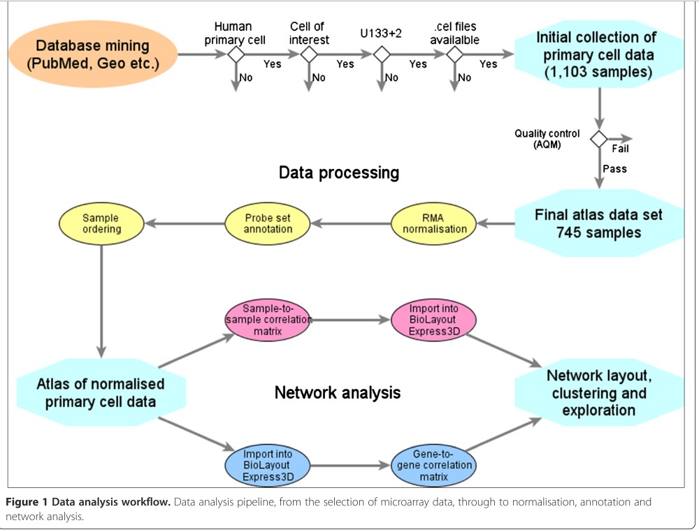
The workflow for producing a reference resource is:
Data structure to be used
The following schematic is from the SummarizedExperiment vignette.

Briefly, a SummarizedExperiment can be treated like a matrix. dim(SE) evaluates to a 2-vector with first element the number of genomic features assayed and second element the number of samples or cells assayed. The syntax SE[r,c] evaluates to a new SummarizedExperiment with rows and columns subset by the predicates r, c. The assay component has rows corresponding to genomic features and columns corresponding to samples or single cells. The colData component manages a table of information about samples or cells. The rowData component manages information about genomic features assayed.
The HPCA SummarizedExperiment
library(BiocNIHIntra)
hd = getHPCAreference()
hd
## class: SummarizedExperiment
## dim: 19363 713
## metadata(0):
## assays(1): logcounts
## rownames(19363): A1BG A1BG-AS1 ... ZZEF1 ZZZ3
## rowData names(0):
## colnames(713): GSM112490 GSM112491 ... GSM92233 GSM92234
## colData names(3): label.main label.fine label.ontThis representation of the HPCA reference has been preprocessed; the paper noted in the help text from ?HumanPrimaryCellAtlasData with the celldex package attached gives details.
The collection of cell types available can be seen with
library(DT)
datatable(as.data.frame(colData(hd)))
The TENx PBMC data
This dataset uses a specialized container called SingleCellExperiment; see the SingleCellExperiment vignette for further details. The schematic is:
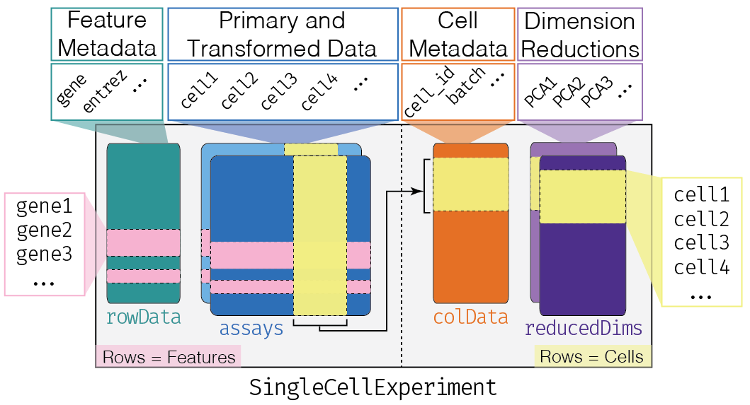
We retrieve the data:
vps = get4kPBMC()
vps
## class: SingleCellExperiment
## dim: 22617 4340
## metadata(0):
## assays(2): counts logcounts
## rownames(22617): FAM138A OR4F5 ... LOC102724250 FAM231C
## rowData names(3): ENSEMBL_ID Symbol_TENx Symbol
## colnames: NULL
## colData names(12): Sample Barcode ... Date_published sizeFactor
## reducedDimNames(0):
## mainExpName: NULL
## altExpNames(0):A nice feature of the Bioconductor approach to dealing with single cell data in SingleCellExperiment is that we can quickly get a display after dimension reduction:
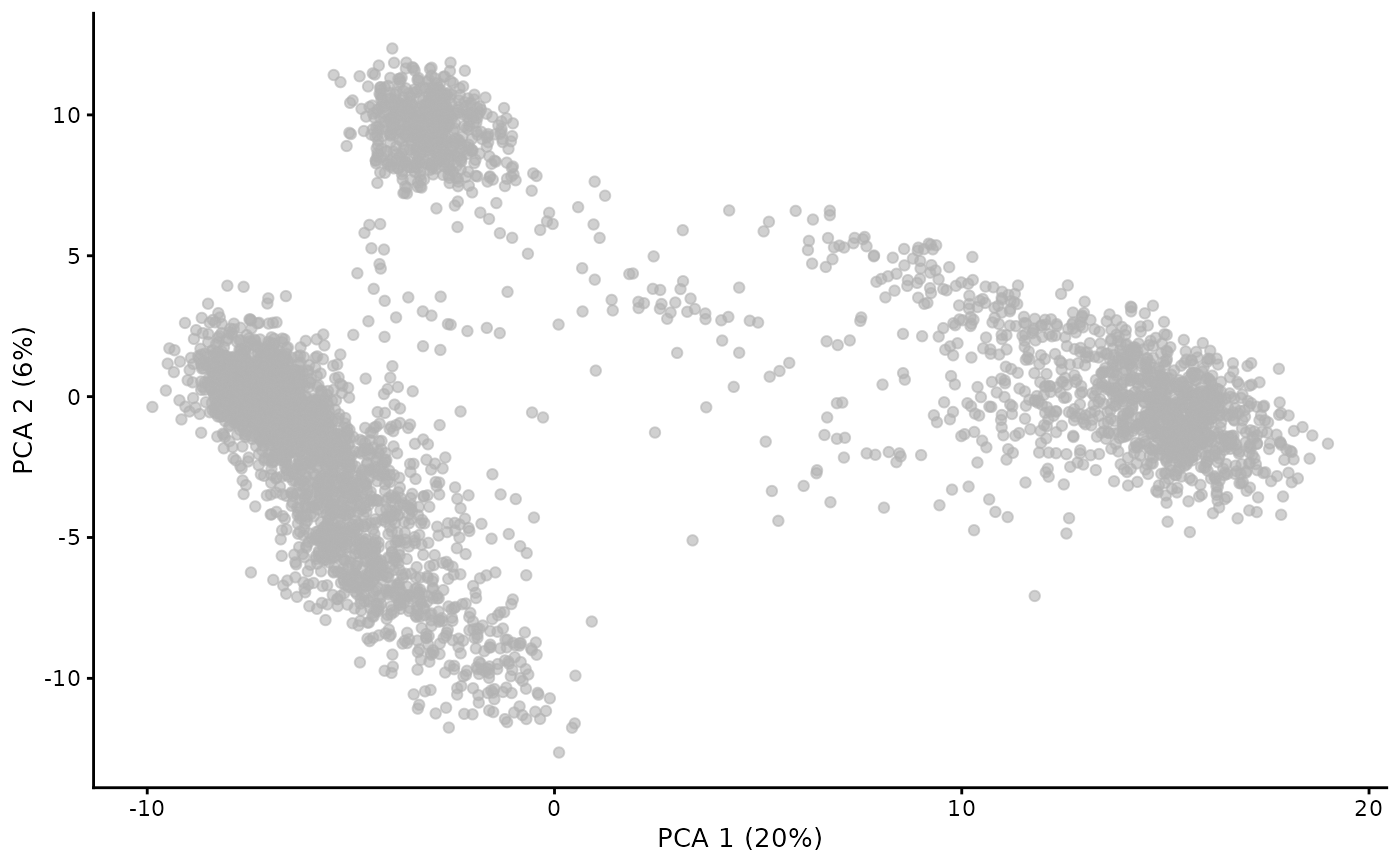 We don’t know the basis of the clustering structure in this display. Perhaps it relates to cell type.
Cell labeling
Now we use the SingleR algorithm with all defaults (see ?SingleR for details) to obtain labels by comparing expression patterns between the PBMC data and the reference.
library(SingleR)
vsing = SingleR(vps, hd, hd$label.main)
vps$label.main = vsing$labels
table(vps$label.main)
##
## B_cell CMP DC GMP
## 606 8 1 2
## Monocyte NK_cell Platelets Pre-B_cell_CD34-
## 1175 218 3 36
## T_cells
## 2291Feature reduction and interactive visualization
We’ll conclude by developing an interactive biplot that shows both the projection to principal components (with a reduced set of genes) and a representation of gene “loadings”, showing contributions of specific genes to the positioning of cells in the principal components projection.
Filter on SD across cells
First we filter to genes with substantial variation across cells – we take the top 20% in the distribution of standard deviations. This produces a SingleCellExperiment vpslim.
Compute approximate PCA
Then we prepare a specific representation of principal components analysis using the irlba procedure for approximate PCA.
set.seed(1234)
mat = t(as.matrix(assay(vpslim,2)))
library(irlba)
apca = prcomp_irlba(mat, 4)
names(apca)
## [1] "scale" "totalvar" "sdev" "rotation" "center" "x"
summary(apca)## Importance of components:
## PC1 PC2 PC3 PC4
## Standard deviation 10.15591 5.79901 4.84326 3.34214
## Proportion of Variance 0.08877 0.02894 0.02019 0.00961
## Cumulative Proportion 0.08877 0.11771 0.13789 0.14751Produce interactive biplot
npl = filtered_biplot(apca, vpslim, nvar=10)## [1] "factor"
## PC1 PC2 ctype
## AAACCTGAGAAGGCCT-1 -16.453882 -1.985401 Monocyte
## AAACCTGAGACAGACC-1 -16.344575 -2.547731 Monocyte
## AAACCTGAGATAGTCA-1 -20.692332 1.447867 Monocyte
## AAACCTGAGCGCCTCA-1 6.163137 2.772246 T_cells
## AAACCTGAGGCATGGT-1 8.950973 -2.216775 T_cells
## AAACCTGCAAGGTTCT-1 8.234260 1.042397 T_cells