A1: Basic Bioconductor packages and data structures for genomics
Vincent J. Carey, stvjc at channing.harvard.edu
May 02, 2023
Source:vignettes/A1_basic.Rmd
A1_basic.RmdGenomic annotation of organisms
Institutionally curated data on model organisms are collected in packages with names starting with org..
library(org.Hs.eg.db)
org.Hs.eg.db
## OrgDb object:
## | DBSCHEMAVERSION: 2.1
## | Db type: OrgDb
## | Supporting package: AnnotationDbi
## | DBSCHEMA: HUMAN_DB
## | ORGANISM: Homo sapiens
## | SPECIES: Human
## | EGSOURCEDATE: 2023-Mar05
## | EGSOURCENAME: Entrez Gene
## | EGSOURCEURL: ftp://ftp.ncbi.nlm.nih.gov/gene/DATA
## | CENTRALID: EG
## | TAXID: 9606
## | GOSOURCENAME: Gene Ontology
## | GOSOURCEURL: http://current.geneontology.org/ontology/go-basic.obo
## | GOSOURCEDATE: 2023-01-01
## | GOEGSOURCEDATE: 2023-Mar05
## | GOEGSOURCENAME: Entrez Gene
## | GOEGSOURCEURL: ftp://ftp.ncbi.nlm.nih.gov/gene/DATA
## | KEGGSOURCENAME: KEGG GENOME
## | KEGGSOURCEURL: ftp://ftp.genome.jp/pub/kegg/genomes
## | KEGGSOURCEDATE: 2011-Mar15
## | GPSOURCENAME: UCSC Genome Bioinformatics (Homo sapiens)
## | GPSOURCEURL:
## | GPSOURCEDATE: 2023-Feb8
## | ENSOURCEDATE: 2023-Feb10
## | ENSOURCENAME: Ensembl
## | ENSOURCEURL: ftp://ftp.ensembl.org/pub/current_fasta
## | UPSOURCENAME: Uniprot
## | UPSOURCEURL: http://www.UniProt.org/
## | UPSOURCEDATE: Wed Mar 15 15:58:07 2023
columns(org.Hs.eg.db)## [1] "ACCNUM" "ALIAS" "ENSEMBL" "ENSEMBLPROT" "ENSEMBLTRANS"
## [6] "ENTREZID" "ENZYME" "EVIDENCE" "EVIDENCEALL" "GENENAME"
## [11] "GENETYPE" "GO" "GOALL" "IPI" "MAP"
## [16] "OMIM" "ONTOLOGY" "ONTOLOGYALL" "PATH" "PFAM"
## [21] "PMID" "PROSITE" "REFSEQ" "SYMBOL" "UCSCKG"
## [26] "UNIPROT"Using AnnotationDbi we can produce data.frames with annotation. We’ll use the gene titin (TTN) to illustrate acquisition of Gene Ontology annotations.
library(AnnotationDbi)
ttnanno = AnnotationDbi::select(org.Hs.eg.db, keys="TTN", keytype="SYMBOL",
  columns=c("ENTREZID", "ENSEMBL", "GENENAME", "GO"))
## 'select()' returned 1:many mapping between keys and columns
head(ttnanno)## SYMBOL ENTREZID ENSEMBL GENENAME GO EVIDENCE ONTOLOGY
## 1 TTN 7273 ENSG00000155657 titin GO:0000794 IDA CC
## 2 TTN 7273 ENSG00000155657 titin GO:0002020 IPI MF
## 3 TTN 7273 ENSG00000155657 titin GO:0003300 IMP BP
## 4 TTN 7273 ENSG00000155657 titin GO:0004674 IDA MF
## 5 TTN 7273 ENSG00000155657 titin GO:0004713 IDA MF
## 6 TTN 7273 ENSG00000155657 titin GO:0005509 IDA MFUsing GO.db through a helper function decode_gotags defined in BiocOV, we can learn aspects of gene function. Here we limit annotations to those identified through “traceable author statements”, “TAS”.
##   SYMBOL ENTREZID         ENSEMBL GENENAME         GO EVIDENCE ONTOLOGY
## 1    TTN     7273 ENSG00000155657    titin GO:0005516      TAS       MF
## 2    TTN     7273 ENSG00000155657    titin GO:0005576      TAS       CC
## 3    TTN     7273 ENSG00000155657    titin GO:0005829      TAS       CC
## 4    TTN     7273 ENSG00000155657    titin GO:0006936      TAS       BP
## 5    TTN     7273 ENSG00000155657    titin GO:0006941      TAS       BP
## 6    TTN     7273 ENSG00000155657    titin GO:0008307      TAS       MF
## 7    TTN     7273 ENSG00000155657    titin GO:0035995      TAS       BP
## 8    TTN     7273 ENSG00000155657    titin GO:0097493      TAS       MF
##         GOID                                               TERM
## 1 GO:0005516                                 calmodulin binding
## 2 GO:0005576                               extracellular region
## 3 GO:0005829                                            cytosol
## 4 GO:0006936                                 muscle contraction
## 5 GO:0006941                        striated muscle contraction
## 6 GO:0008307                   structural constituent of muscle
## 7 GO:0035995                        detection of muscle stretch
## 8 GO:0097493 structural molecule activity conferring elasticity
Genomic sequence and genomic coordinates
The full sequences of model organisms are available using Biostrings and BSgenome resources.
library(BSgenome.Hsapiens.UCSC.hg19)
Hsapiens
## | BSgenome object for Human
## | - organism: Homo sapiens
## | - provider: UCSC
## | - genome: hg19
## | - release date: June 2013
## | - 298 sequence(s):
## | chr1 chr2 chr3
## | chr4 chr5 chr6
## | chr7 chr8 chr9
## | chr10 chr11 chr12
## | chr13 chr14 chr15
## | ... ... ...
## | chr19_gl949749_alt chr19_gl949750_alt chr19_gl949751_alt
## | chr19_gl949752_alt chr19_gl949753_alt chr20_gl383577_alt
## | chr21_gl383578_alt chr21_gl383579_alt chr21_gl383580_alt
## | chr21_gl383581_alt chr22_gl383582_alt chr22_gl383583_alt
## | chr22_kb663609_alt
## |
## | Tips: call 'seqnames()' on the object to get all the sequence names, call
## | 'seqinfo()' to get the full sequence info, use the '$' or '[[' operator to
## | access a given sequence, see '?BSgenome' for more information.
substr(Hsapiens$chr1, 1e6, 2e6-1)## 1000000-letter DNAString object
## seq: TGGGCACAGCCTCACCCAGGAAAGCAGCTGGGGGTC...GGGCAGTCCAGGACATTCACCTTGAGACCTGGCCTTUCSC gene coordinates
Gene models are available in the TxDb series of packages.
library(TxDb.Hsapiens.UCSC.hg19.knownGene)
txdb = TxDb.Hsapiens.UCSC.hg19.knownGene
txdb
## TxDb object:
## # Db type: TxDb
## # Supporting package: GenomicFeatures
## # Data source: UCSC
## # Genome: hg19
## # Organism: Homo sapiens
## # Taxonomy ID: 9606
## # UCSC Table: knownGene
## # Resource URL: http://genome.ucsc.edu/
## # Type of Gene ID: Entrez Gene ID
## # Full dataset: yes
## # miRBase build ID: GRCh37
## # transcript_nrow: 82960
## # exon_nrow: 289969
## # cds_nrow: 237533
## # Db created by: GenomicFeatures package from Bioconductor
## # Creation time: 2015-10-07 18:11:28 +0000 (Wed, 07 Oct 2015)
## # GenomicFeatures version at creation time: 1.21.30
## # RSQLite version at creation time: 1.0.0
## # DBSCHEMAVERSION: 1.1
g = genes(txdb)
g
## GRanges object with 23056 ranges and 1 metadata column:
## seqnames ranges strand | gene_id
## <Rle> <IRanges> <Rle> | <character>
## 1 chr19 58858172-58874214 - | 1
## 10 chr8 18248755-18258723 + | 10
## 100 chr20 43248163-43280376 - | 100
## 1000 chr18 25530930-25757445 - | 1000
## 10000 chr1 243651535-244006886 - | 10000
## ... ... ... ... . ...
## 9991 chr9 114979995-115095944 - | 9991
## 9992 chr21 35736323-35743440 + | 9992
## 9993 chr22 19023795-19109967 - | 9993
## 9994 chr6 90539619-90584155 + | 9994
## 9997 chr22 50961997-50964905 - | 9997
## -------
## seqinfo: 93 sequences (1 circular) from hg19 genomeThe genes function returns a GenomicRanges instance. We can add gene symbols using AnnotationDbi and org.Hs.eg.db.
smap = AnnotationDbi::select(org.Hs.eg.db,
   keys=g$gene_id, keytype="ENTREZID", columns="SYMBOL")
## 'select()' returned 1:1 mapping between keys and columns
g$gene_symbol = smap$SYMBOL
head(g)
## GRanges object with 6 ranges and 2 metadata columns:
## seqnames ranges strand | gene_id gene_symbol
## <Rle> <IRanges> <Rle> | <character> <character>
## 1 chr19 58858172-58874214 - | 1 A1BG
## 10 chr8 18248755-18258723 + | 10 NAT2
## 100 chr20 43248163-43280376 - | 100 ADA
## 1000 chr18 25530930-25757445 - | 1000 CDH2
## 10000 chr1 243651535-244006886 - | 10000 AKT3
## 100008586 chrX 49217763-49233491 + | 100008586 GAGE12F
## -------
## seqinfo: 93 sequences (1 circular) from hg19 genomeThe genomic coordinates for genes of interest can now be retrieved from g.
ttnco = g[ which(g$gene_symbol == "TTN") ]
ttnco
## GRanges object with 1 range and 2 metadata columns:
## seqnames ranges strand | gene_id gene_symbol
## <Rle> <IRanges> <Rle> | <character> <character>
## 7273 chr2 179390717-179672150 - | 7273 TTN
## -------
## seqinfo: 93 sequences (1 circular) from hg19 genomeAnd the coding sequence can be extracted from Hsapiens.
## 281434-letter DNAString object
## seq: TTTGAGGTGCAGATAGCTTGCTTTATTTTGTTGTTA...TACACCCGAGGCGAGGCTGGGAATGCACGACTGCTC
Ensemble gene coordinates
The EnsDb. packages provide richer annotation through the genes method.
library(EnsDb.Hsapiens.v75) # same as hg19## Loading required package: ensembldb## Loading required package: AnnotationFilter##
## Attaching package: 'ensembldb'## The following object is masked from 'package:dplyr':
##
## filter## The following object is masked from 'package:stats':
##
## filter
genes(EnsDb.Hsapiens.v75)## GRanges object with 64102 ranges and 6 metadata columns:
## seqnames ranges strand | gene_id
## <Rle> <IRanges> <Rle> | <character>
## ENSG00000223972 1 11869-14412 + | ENSG00000223972
## ENSG00000227232 1 14363-29806 - | ENSG00000227232
## ENSG00000243485 1 29554-31109 + | ENSG00000243485
## ENSG00000237613 1 34554-36081 - | ENSG00000237613
## ENSG00000268020 1 52473-54936 + | ENSG00000268020
## ... ... ... ... . ...
## ENSG00000224240 Y 28695572-28695890 + | ENSG00000224240
## ENSG00000227629 Y 28732789-28737748 - | ENSG00000227629
## ENSG00000237917 Y 28740998-28780799 - | ENSG00000237917
## ENSG00000231514 Y 28772667-28773306 - | ENSG00000231514
## ENSG00000235857 Y 59001391-59001635 + | ENSG00000235857
## gene_name gene_biotype seq_coord_system symbol
## <character> <character> <character> <character>
## ENSG00000223972 DDX11L1 pseudogene chromosome DDX11L1
## ENSG00000227232 WASH7P pseudogene chromosome WASH7P
## ENSG00000243485 MIR1302-10 lincRNA chromosome MIR1302-10
## ENSG00000237613 FAM138A lincRNA chromosome FAM138A
## ENSG00000268020 OR4G4P pseudogene chromosome OR4G4P
## ... ... ... ... ...
## ENSG00000224240 CYCSP49 pseudogene chromosome CYCSP49
## ENSG00000227629 SLC25A15P1 pseudogene chromosome SLC25A15P1
## ENSG00000237917 PARP4P1 pseudogene chromosome PARP4P1
## ENSG00000231514 FAM58CP pseudogene chromosome FAM58CP
## ENSG00000235857 CTBP2P1 pseudogene chromosome CTBP2P1
## entrezid
## <list>
## ENSG00000223972 100287596,100287102
## ENSG00000227232 100287171,653635
## ENSG00000243485 100422919,100422834,100422831,...
## ENSG00000237613 654835,645520,641702
## ENSG00000268020 <NA>
## ... ...
## ENSG00000224240 <NA>
## ENSG00000227629 <NA>
## ENSG00000237917 <NA>
## ENSG00000231514 <NA>
## ENSG00000235857 <NA>
## -------
## seqinfo: 273 sequences (1 circular) from GRCh37 genomeInteractive visualization of genes
The TnT includes javascript facilities for interactively visualizing genomes and data collected in genomic coordinates. We’ll show the context of TTN. If you have a click-wheel it can be used to zoom in and out, and to pan across the genome.
gene = genes(EnsDb.Hsapiens.v75)
ensGeneTrack <- TnT::FeatureTrack(gene, tooltip = as.data.frame(gene),
                       names = paste(gene$symbol, " (", gene$gene_biotype, ")", sep = ""),
                       color = TnT::mapcol(gene$gene_biotype, palette.fun = grDevices::rainbow))
inir = GRanges("2", IRanges(179380000, 179490000))
TnTGenome(ensGeneTrack, view.range = inir)
Exercises
Tabulating annotation for a region of interest
The following function obtains a data.frame with information about a 10Mb segment of chromosome 2.
ginfo = function(chr="2", start=170e6, end=180e6) {
  g = ensembldb::genes(EnsDb.Hsapiens.v75)
  targ = GenomicRanges::GRanges(chr, IRanges::IRanges(start, end))
  as.data.frame(IRanges::subsetByOverlaps(g, targ))
}
tab = ginfo()
The average number of protein-coding genes per megabase in this region can be obtained as
## [1] 7.195026What is the average number of protein-coding genes per megabase for all of chromosome 2?
- You will run the
ginfofunction with different arguments. - The lengths of chromosomes can be obtained via
seqinfo(Hsapiens).
Exploring annotation on cellular localization of gene activity
Here is a helper function for tabulating annotation for a gene identified by symbol.
myanno = function(gene_symbol="BRCA2")
    AnnotationDbi::select(org.Hs.eg.db, keys=gene_symbol, keytype="SYMBOL",
       columns=c("ENTREZID", "ENSEMBL", "GENENAME", "GO"))
dim(myanno())
## 'select()' returned 1:many mapping between keys and columns## [1] 56 7We use the CC (cellular component) subontology of GO to see what components BRCA2 has been annotated to:
library(DT)
brtab = myanno("BRCA2") |> dplyr::filter(ONTOLOGY=="CC") |> decode_gotags()
datatable(brtab)
Note that the same component can be annotated on the basis of different evidence codes.
Find the cellular components annotated for gene ORMDL3, and for genes of your choice.
Coordinated data structures for multisample genomics
SummarizedExperiment
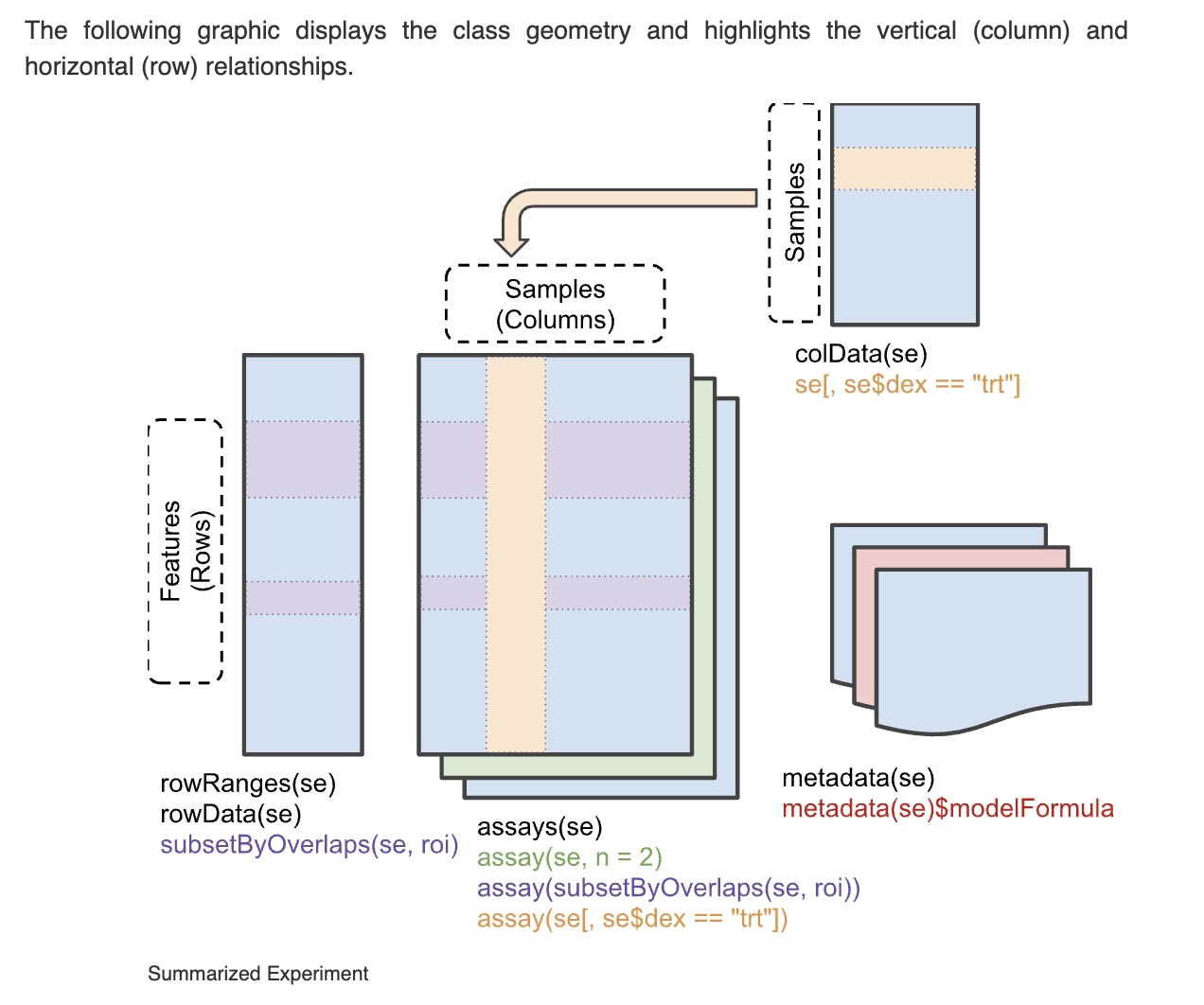
Relative to typical volumes and arrangements of data in scientific studies, genomic studies are distinguished by very large numbers of features collected per sample. Measurements often fall into two classes.
- Matrix-like structures store the collection of molecular assay outputs, involving one or more digital measurements per genomic feature. This component is referred to as “Assay”. - In addition to the assay outputs, a data table is needed to store information on sample characteristics. This component is referred to as “colData”.
Additional metadata on assay features and on the experiment as a whole must be accommodated, “tightly bound” with all the other information so that crucial information about context and interpretation do not scatter away.
A schematic view of the “SummarizedExperiment” that collects these information components is here:
An example can be obtained using ExperimentHub. This SummarizedExperiment instance collects all the non-tumor tissue samples in The Cancer Genome Atlas (TCGA), and labels them with the organ in which a tumor was sampled.
library(ExperimentHub)
eh = ExperimentHub()
tnorm = eh[["EH1044"]]
tnorm
## class: SummarizedExperiment
## dim: 23368 741
## metadata(0):
## assays(1): NormalRaw
## rownames(23368): 1/2-SBSRNA4 A1BG ... ZZZ3 tAKR
## rowData names(0):
## colnames(741): TCGA-K4-A3WV-11A-21R-A22U-07
## TCGA-49-6742-11A-01R-1858-07 ... TCGA-BH-A0H5-11A-62R-A115-07
## TCGA-22-5489-11A-01R-1635-07
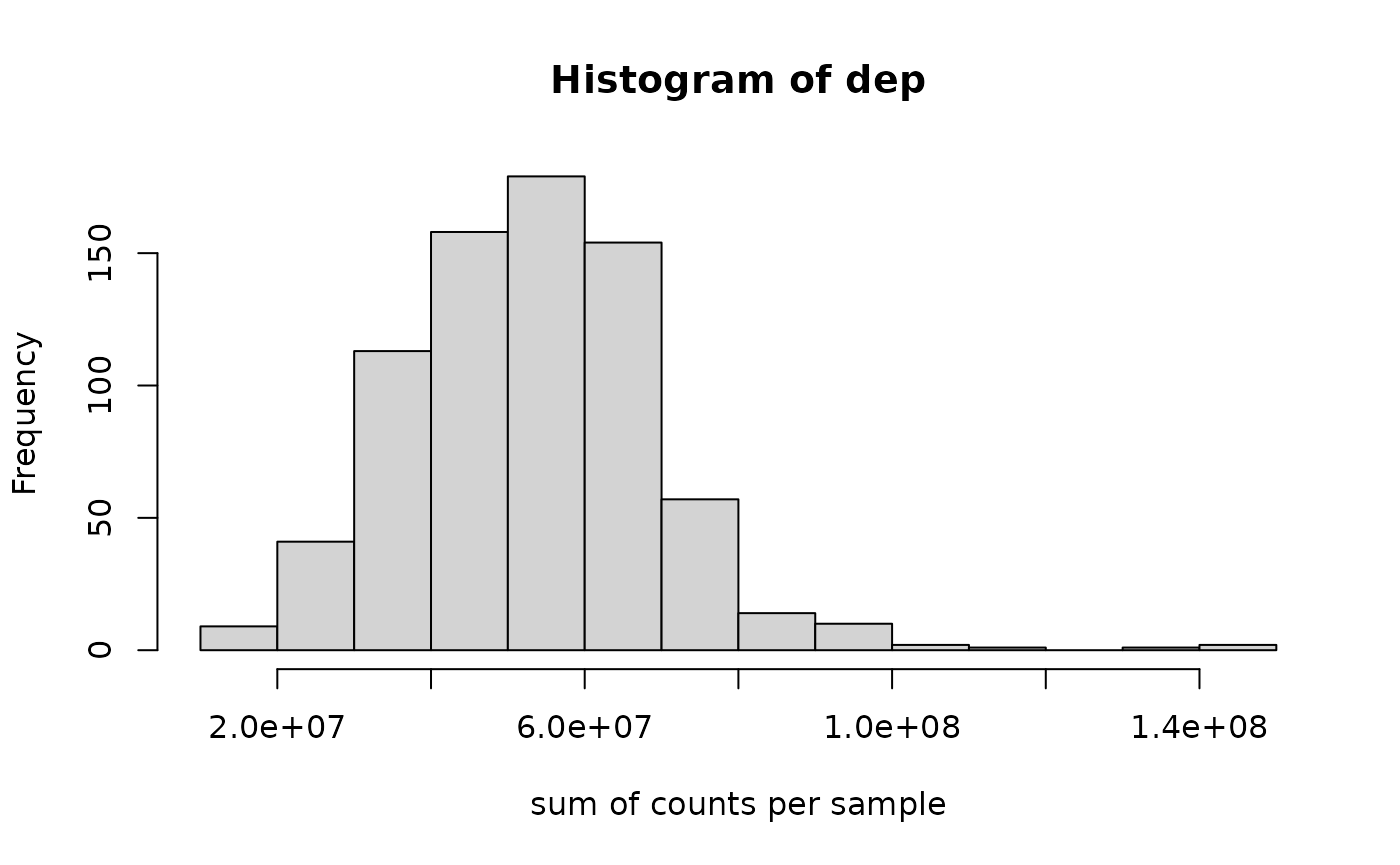
## colData names(2): sample typeWe compute the sequencing depth per sample using
The tissue type with smallest value of depth is:
tnorm$type[ which.min(dep) ]## [1] UCEC
## 24 Levels: BLCA BRCA CESC CHOL COAD ESCA GBM HNSC KICH KIRC KIRP LIHC ... UCECExercises
Most deeply sequenced
Three samples have depth values exceeding 120,000,000. What type(s) of tissue are they derived from?
A gene with bimodally distributed expression
Examine the output of
hist(as.numeric(assay(tnorm["A1BG",])))From what tissue type are the samples with very high levels of A1BG derived? Check the NCBI report on this gene to explain this finding.
SingleCellExperiment
The explosion of interest in single-cell RNA-seq has inspired the extension of the SummarizedExperiment design to simplify common tasks employed with single-cell studies.
A schematic of the SingleCellExperiment class is:
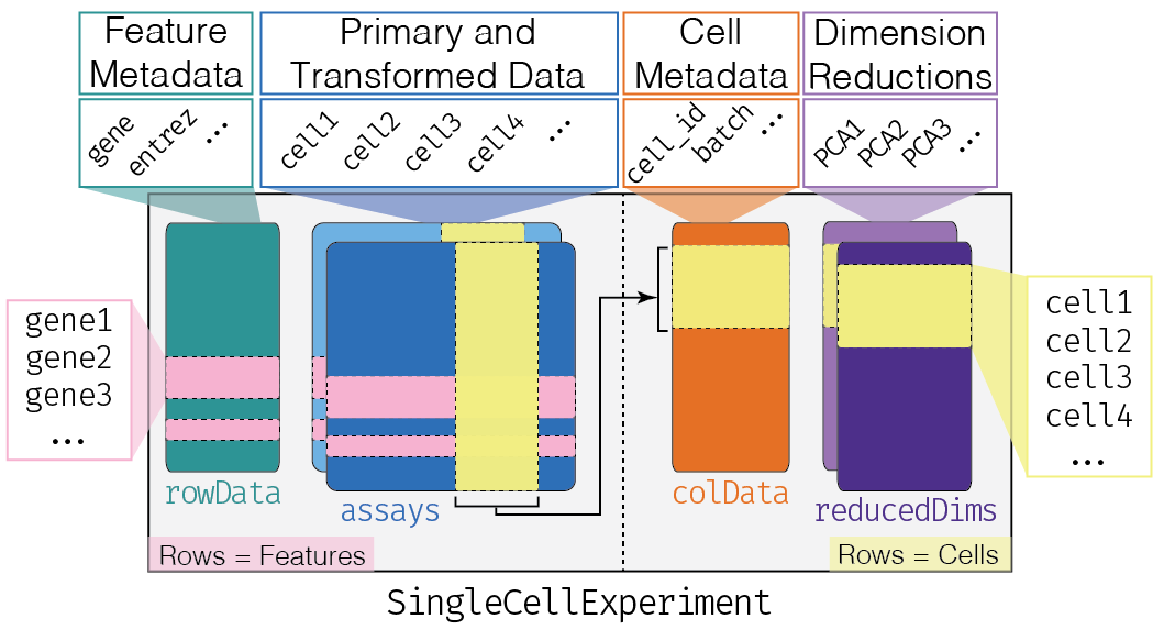
SCE schematic
Predicting cell type using reference expression data
These illustrations are taken from the introduction to the SingleR book.
The “Human Primary Cell Atlas” records expression patterns for sorted cells. The cell type distributions are tabulated here, drilling down on “T cells” for subtypes.
library(celldex)
ref.data <- HumanPrimaryCellAtlasData(ensembl=TRUE)
## Warning: Unable to map 1470 of 19363 requested IDs.
ref.data## class: SummarizedExperiment
## dim: 17893 713
## metadata(0):
## assays(1): logcounts
## rownames(17893): ENSG00000121410 ENSG00000268895 ... ENSG00000159840
## ENSG00000074755
## rowData names(0):
## colnames(713): GSM112490 GSM112491 ... GSM92233 GSM92234
## colData names(3): label.main label.fine label.ont
table(ref.data$label.main)##
## Astrocyte B_cell BM
## 2 26 7
## BM & Prog. Chondrocytes CMP
## 1 8 2
## DC Embryonic_stem_cells Endothelial_cells
## 88 17 64
## Epithelial_cells Erythroblast Fibroblasts
## 16 8 10
## Gametocytes GMP Hepatocytes
## 5 2 3
## HSC_-G-CSF HSC_CD34+ iPS_cells
## 10 6 42
## Keratinocytes Macrophage MEP
## 25 90 2
## Monocyte MSC Myelocyte
## 60 9 2
## Neuroepithelial_cell Neurons Neutrophils
## 1 16 21
## NK_cell Osteoblasts Platelets
## 5 15 5
## Pre-B_cell_CD34- Pro-B_cell_CD34+ Pro-Myelocyte
## 2 2 2
## Smooth_muscle_cells T_cells Tissue_stem_cells
## 16 68 55
table(ref.data$label.fine[ref.data$label.main=="T_cells"])##
## T_cell:CCR10-CLA+1,25(OH)2_vit_D3/IL-12 T_cell:CCR10+CLA+1,25(OH)2_vit_D3/IL-12
## 1 1
## T_cell:CD4+ T_cell:CD4+_central_memory
## 12 5
## T_cell:CD4+_effector_memory T_cell:CD4+_Naive
## 4 6
## T_cell:CD8+ T_cell:CD8+_Central_memory
## 16 3
## T_cell:CD8+_effector_memory T_cell:CD8+_effector_memory_RA
## 4 4
## T_cell:CD8+_naive T_cell:effector
## 4 4
## T_cell:gamma-delta T_cell:Treg:Naive
## 2 2Unlabeled single-cell expression patterns were assayed on 4000 PBMCs using the TENx platform. We acquire the SingleCellExperiment:
library(TENxPBMCData)
new.data <- TENxPBMCData("pbmc4k")
The unlabeled cells are compared to reference and labels are inferred using the method in
     Aran D, Looney AP, Liu L et al. (2019). Reference-based analysis
     of lung single-cell sequencing reveals a transitional profibrotic
     macrophage. _Nat. Immunology_ 20, 163–172.
Notice that by using plotly for the visualization below, we can hover over the graph in the browser to see the cell type in a textual widget.
library(plotly)
library(SingleR)
predictions <- SingleR(test=new.data, assay.type.test=1,
    ref=ref.data, labels=ref.data$label.main)
table(predictions$labels)
##
## B_cell CMP DC GMP
## 606 8 1 2
## Monocyte NK_cell Platelets Pre-B_cell_CD34-
## 1164 217 3 46
## T_cells
## 2293Exercises
B cell subtypes
Modify the code below to obtain labels and counts of B cell subtypes in the Human Primary Cell Atlas.
table(ref.data$label.fine[ref.data$label.main=="T_cells"])Visualizing subtypes
No coding. How would you modify the code below to color the display by finer-grained cell classifications?
library(plotly)
library(SingleR)
predictions <- SingleR(test=new.data, assay.type.test=1,
ref=ref.data, labels=ref.data$label.main)
table(predictions$labels)
library(scater)
nn = logNormCounts(new.data)
nn = runPCA(nn)
nn$type = predictions$labels
ans = plotPCA(nn,colour_by="type")
ggplotly(ans)Dynamic visualization
This method needs some help in mapping colors to textual labels.
We’ll use the R CRANpkg("threejs") package to project from PC2-4 to the screen with interactive rotation support.
First we set up a color palette:
mycol = palette.colors(26, "Polychrome 36")
head(mycol)
## darkpurplishgray purplishwhite vividred vividpurple
## "#5A5156" "#E4E1E3" "#F6222E" "#FE00FA"
## vividyellowishgreen strongpurplishblue
## "#16FF32" "#3283FE"Now obtain assignments of colors to cells.
colinds = as.numeric(factor(nn$type))
colors = mycol[colinds]
Finally produce the interactive display.
library(threejs)
scatterplot3js( reducedDims(nn)$PCA[,2:4] ,color=unname(colors), size=.4)
MultiAssayExperiment
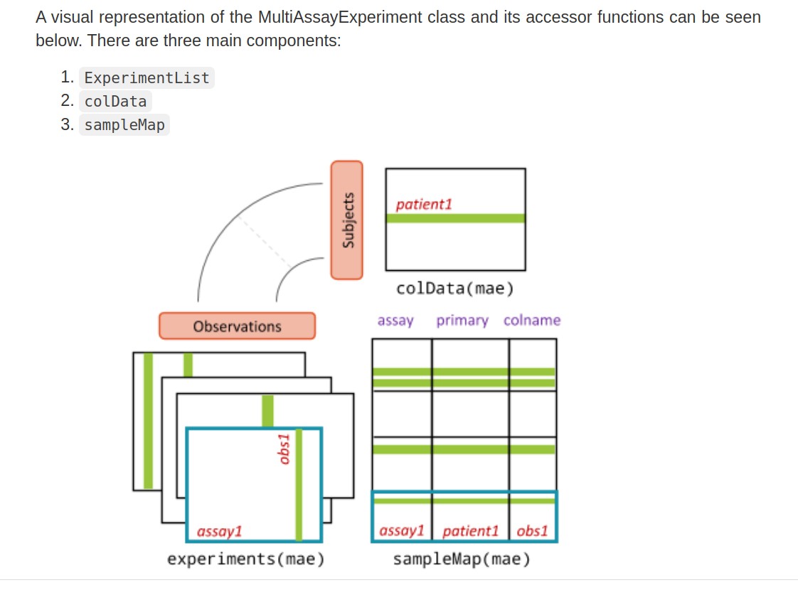
MAE
- The colData provides data about the patients, cell lines, or other biological units, with one row per unit and one column per variable.
- The experiments are a list of assay datasets of arbitrary class, with one column per observation.
- The sampleMap links a single table of patient data (colData) to a list of experiments via a simple but powerful table of experiment:patient edges (relationships), that can be created automatically in simple cases or in a spreadsheet if assay-specific sample identifiers are used. sampleMap relates each column (observation) in the assays (experiments) to exactly one row (biological unit) in colData; however, one row of colData may map to zero, one, or more columns per assay, allowing for missing and replicate assays. Green stripes indicate a mapping of one subject to multiple observations across experiments.
We will work with a MultiAssayExperiment in the B1 vignette.