BiocSfaira overview

Introduction

This works through some of the components of the Sfaira UI tutorial notebook.

Setup

Install via BiocManager::install('vjcitn/BiocSfaira')

This uses a simple configuration approach specified in DESCRIPTION to acquire necessary python infrastructure. As the sfaira code is run, additional infrastructure may be loaded by python functions. Typically caching is used so these are one-time events.

set.seed(123)
library(BiocSfaira)
library(zellkonverter)
library(SingleCellExperiment)
library(plotly)

Resources

Sfaira provides embeddings (projections from high-dimensional expression quantifications to low-dimension ‘latent spaces’) and type-assignment resources, all tissue- and organism-specific.

ui = sfaira_ui()
ems = ui$zoo_embedding$available_model_ids
sample(ems, size=10)

##  [1] "embedding_mouse-heart-nmf-0.1-0.1_theislab"       
##  [2] "embedding_mouse-spleen-nmf-0.1-0.1_theislab"      
##  [3] "embedding_mouse-mammarygland-nmf-0.2-0.1_theislab"
##  [4] "embedding_human-blood-linear-0.2-0.1_theislab"    
##  [5] "embedding_mouse-placenta-nmf-0.2-0.1_theislab"    
##  [6] "embedding_mouse-liver-linear-0.2-0.1_theislab"    
##  [7] "embedding_human-kidney-linear-0.1-0.1_theislab"   
##  [8] "embedding_human-trachea-linear-0.2-0.1_theislab"  
##  [9] "embedding_human-heart-nmf-0.1-0.1_theislab"       
## [10] "embedding_mouse-uterus-ae-0.1-0.1_theislab"

We’ll pick an embedding in the next section.

cts = ui$zoo_celltype$available_model_ids
sample(cts, size=10)

##  [1] "celltype_mouse-heart-marker-0.0.1-0.1_theislab"      
##  [2] "celltype_mouse-spleen-mlp-0.1.2-0.1_theislab"        
##  [3] "celltype_human-trachea-mlp-0.1.2-0.1_theislab"       
##  [4] "celltype_human-ureter-marker-0.0.1-0.1_theislab"     
##  [5] "celltype_mouse-urinarybladder-mlp-0.1.1-0.1_theislab"
##  [6] "celltype_human-ureter-mlp-0.0.1-0.1_theislab"        
##  [7] "celltype_mouse-muscleorgan-mlp-0.0.1-0.1_theislab"   
##  [8] "celltype_human-uterus-mlp-0.1.3-0.1_theislab"        
##  [9] "celltype_human-spinalcord-mlp-0.1.3-0.1_theislab"    
## [10] "celltype_human-eye-mlp-0.0.1-0.1_theislab"

The models are either multilayer perceptron or ‘marker’-based. This is tersely explained in the Genome Biology paper.

Multilayer perceptron model We used dense layer stacks (multilayer perceptron) to predict cell types from gene ex- pression data. An example multilayer perceptron for cell type prediction used in this study was trained on all protein coding genes from either mouse or human, had one hidden layer of the size (128), was trained without L1 and L2 penalties on the parame- ters, and with a selu activation function.

Marker model We defined a marker gene-dominated model to predict cell types from gene expression data. In this model, a sigmoid function based on a gene-specific linear embedding of the gene expression values models an expression threshold. After this gene-wise em- bedding, a fully connected layer pools information from all genes to the cell type prediction.

Using an autoencoder trained on blood to classify PBMCs

First we use the UI components to pick our resources.

ui$zoo_embedding$model_id = "embedding_human-blood-ae-0.2-0.1_theislab"
ui$zoo_celltype$model_id = "celltype_human-blood-mlp-0.1.3-0.1_theislab"

We use scanpy’s datasets library to get an AnnData representation of expression patterns for around 3000 PBMCs.

sc = scanpy_ref()
p = sc$datasets$pbmc3k()

Now we load the AnnData into the UI component and run the embedding and type prediction procedures.

ui$load_data(p, gene_symbol_col='index', gene_ens_col='gene_ids')
ui$load_model_celltype()
ui$load_model_embedding()
ui$predict_all() 
ui$data$adata

## AnnData object with n_obs × n_vars = 2700 × 19973
##     obs: 'assay_sc', 'assay_differentiation', 'assay_type_differentiation', 'bio_sample', 'cell_line', 'cell_type', 'development_stage', 'disease', 'ethnicity', 'id', 'individual', 'organ', 'organism', 'sex', 'state_exact', 'sample_source', 'tech_sample', 'assay_sc_ontology_term_id', 'cell_line_ontology_term_id', 'cell_type_ontology_term_id', 'development_stage_ontology_term_id', 'disease_ontology_term_id', 'ethnicity_ontology_term_id', 'organ_ontology_term_id', 'organism_ontology_term_id', 'sex_ontology_term_id', 'celltypes_sfaira', 'celltypes_sfaira_id'
##     var: 'ensembl', 'gene_symbol'
##     uns: 'mapped_features', 'annotated', 'author', 'default_embedding', 'doi_journal', 'doi_preprint', 'download_url_data', 'download_url_meta', 'normalization', 'primary_data', 'title', 'year', 'load_raw', 'remove_gene_version', 'assay_sc', 'assay_differentiation', 'assay_type_differentiation', 'cell_line', 'cell_type', 'development_stage', 'disease', 'ethnicity', 'id', 'organ', 'organism', 'sex', 'state_exact', 'sample_source'
##     obsm: 'X_sfaira'

This new AnnData instance can be used to explore the embedding and the labeling. But we’ll do it with SingleCellExperiment.

Converting and exploring

library(zellkonverter)
sce = AnnData2SCE(ui$data$adata)

## Warning: 'X' matrix does not support transposition and has been
## skipped

sce

## class: SingleCellExperiment 
## dim: 19973 2700 
## metadata(28): mapped_features annotated ... state_exact sample_source
## assays(1): X
## rownames(19973): ENSG00000000003 ENSG00000000005 ... ENSG00000288674
##   ENSG00000288675
## rowData names(2): ensembl gene_symbol
## colnames(2700): AAACATACAACCAC-1 AAACATTGAGCTAC-1 ... TTTGCATGAGAGGC-1
##   TTTGCATGCCTCAC-1
## colData names(28): assay_sc assay_differentiation ... celltypes_sfaira
##   celltypes_sfaira_id
## reducedDimNames(1): X_sfaira
## mainExpName: NULL
## altExpNames(0):

dim(reducedDim(sce))

## [1] 2700   64

tail(sort(table(sce$celltypes_sfaira)))

## 
## CD16-negative, CD56-bright natural killer cell, human 
##                                                   164 
##                                          naive B cell 
##                                                   230 
##  naive thymus-derived CD4-positive, alpha-beta T cell 
##                                                   266 
##       effector memory CD8-positive, alpha-beta T cell 
##                                                   338 
##        central memory CD4-positive, alpha-beta T cell 
##                                                   518 
##                      CD14-low, CD16-positive monocyte 
##                                                   638

The embedding has 64 columns:

pairs(reducedDim(sce)[,1:4])

pairs(reducedDim(sce)[,61:64])

The tutorial suggests the following steps for visualization:

sc$pp$neighbors(ui$data$adata, use_rep="X_sfaira")
sc$tl$umap(ui$data$adata)

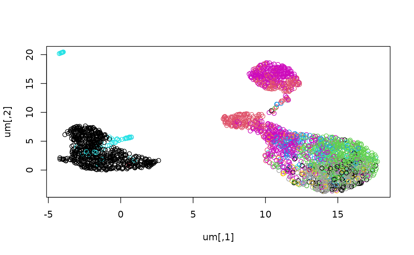
The previous commands add components to the AnnData representation. We extract the UMAP to R and plot, coloring by labels.

um = ui$data$adata$obsm["X_umap"] 
ct = ui$data$adata$obs$celltypes_sfaira 
plot(um, col=as.numeric(factor(ct)))

We can use R’s visualization tools now to help explore interactively. Exercise: make an interactive visualization using ggplotly.

Solution:

library(ggplot2)
library(plotly)
umdf = data.frame(um, type=ct)
gp2 = ggplot(umdf, aes(x=X1, y=X2, text=type, colour=type)) + geom_point()
ggplotly(gp2)

Exercise: Produce a 3 dimensional UMAP projection and use threejs to produce a rotatable 3-d visualization.

Vincent J. Carey, stvjc at channing.harvard.edu

July 11, 2023

Introduction

Setup

Resources

Using an autoencoder trained on blood to classify PBMCs

Converting and exploring