Simba4bioc: interfacing SIMBA’s graph embedding methods to Bioconductor
Vincent J. Carey, stvjc at channing.harvard.edu
October 09, 2023
Source:vignettes/Simba4Bioc.Rmd
Simba4Bioc.RmdIntroduction
SIMBA (paper link) (github) provides methods for “graph embeddings” of relationships between elements assayed in multimodal single cell experiments. The main software stack is written in Python. This package uses basilisk to simplify use of the SIMBA methods in R/Bioconductor.
Motivating illustration
The key component of the package is the “pinned” simba python module. Most of what is computed in using SIMBA graph embeddings is defined in this module.
library(Simba4Bioc)
sref = simba_ref()
names(sref)
## [1] "AnnData" "datasets" "json" "load_graph_stats"
## [5] "load_pbg_config" "os" "Path" "pd"
## [9] "pl" "plotting" "pp" "preprocessing"
## [13] "read_10x_h5" "read_csv" "read_embedding" "read_excel"
## [17] "read_h5ad" "read_hdf" "read_loom" "read_mtx"
## [21] "read_text" "read_umi_tools" "read_zarr" "readwrite"
## [25] "settings" "sys" "tables" "tl"
## [29] "tools" "write_bed"Acquiring demonstration data
The “3k PBMC” dataset from TENx is a common resource for demonstrations. We have a compressed version of it and the get_ function will uncompress and return the path of the h5ad (AnnData) representation. We then use the read_h5ad method from simba to access the dataset.
p3k = get_10x3kpbmc_path(overwrite=TRUE)
pp = sref$read_h5ad(p3k)
pp is now a proper AnnData instance.
pp## AnnData object with n_obs × n_vars = 2700 × 32738
## obs: 'celltype'
## var: 'gene_ids'
names(pp)## [1] "chunk_X" "chunked_X"
## [3] "concatenate" "copy"
## [5] "file" "filename"
## [7] "is_view" "isbacked"
## [9] "isview" "layers"
## [11] "n_obs" "n_vars"
## [13] "obs" "obs_keys"
## [15] "obs_names" "obs_names_make_unique"
## [17] "obs_vector" "obsm"
## [19] "obsm_keys" "obsp"
## [21] "raw" "rename_categories"
## [23] "shape" "strings_to_categoricals"
## [25] "T" "to_df"
## [27] "to_memory" "transpose"
## [29] "uns" "uns_keys"
## [31] "var" "var_keys"
## [33] "var_names" "var_names_make_unique"
## [35] "var_vector" "varm"
## [37] "varm_keys" "varp"
## [39] "write" "write_csvs"
## [41] "write_h5ad" "write_loom"
## [43] "write_zarr" "X"
pp['X'][1:3,1:3]## 3 x 3 sparse Matrix of class "dgRMatrix"
##
## [1,] . . .
## [2,] . . .
## [3,] . . .Building and exploring the graph embedding
Code and output
This sequence of commands will filter genes and build a graph of genes and cells as nodes and weighted edges defined by discretized expression measures. (See tools/_general.py in the simba modules for details on the discretization procedure.)
bb = basic_preproc(pp, simba_ref=sref)
gg = build_and_train_pbg( bb, simba_ref=sref )
dict = sref$read_embedding()
dict is list containing a pair of AnnData instances named ‘C’ and ‘G’ corresponding to cell and gene embeddings respectively.
Embedding layout
Before we start exploring the embeddings numerically, let’s see what kinds of data elements are involved. SIMBA uses the PyTorch BigGraph framework.
For the operations noted above, the graph data take the following form:
pbg
└── graph0
    ├── entity_alias.txt
    ├── graph_stats.json
    ├── input
    │   ├── edge
    │   │   └── edges_0_0.h5
    │   └── entity
    │       ├── entity_count_C_0.txt
    │       ├── entity_count_G_0.txt
    │       ├── entity_names_C_0.json
    │       └── entity_names_G_0.json
    ├── model
    │   ├── checkpoint_version.txt
    │   ├── config.json
    │   ├── embeddings_C_0.v10.h5
    │   ├── embeddings_G_0.v10.h5
    │   ├── model.v10.h5
    │   └── training_stats.json
    └── pbg_graph.txt
The folder names graph0 and model are arbitrary, set as defaults in the build_and_train_pbg function. The graph0/model/embeddings... HDF5 files hold the coordinates of cells and genes in the graph-derived latent spaces. Thus an invocation of rhdf5::h5read on the embeddings_C_0.v10.h5 file will produce a 50 x 2700 matrix of FLOAT.
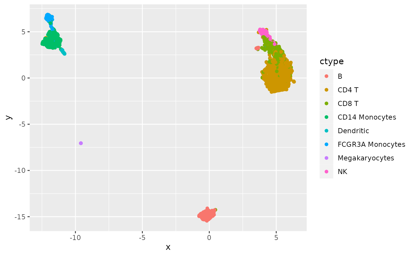
Figure 2b: UMAP for cell embedding
To reproduce Figure 2b of the SIMBA paper without recomputing the graph embedding we have stored the cell embedding in the package, for retrieval using read_h5ad(get_3k_cell_emb()). The cell type labels in the initial AnnData instance pp computed above need to be reorganized.
cemb = sref$read_h5ad(get_3k_cell_emb())
cemb$obs$tmp = pp[cemb$obs_names]$obs[["celltype"]]
names(cemb$obs) = "celltype"
library(uwot)
set.seed(1234)
cumap = umap(cemb['X'])
library(ggplot2)
mydf = data.frame(x=cumap[,1], y=cumap[,2],
   ctype=cemb$obs$celltype)
ggplot(mydf, aes(x=x,y=y,colour=ctype)) + geom_point()
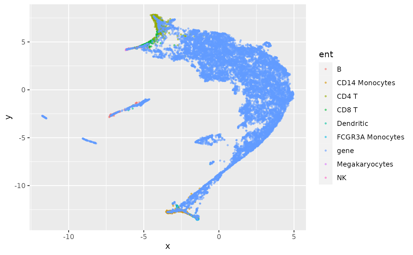
Figure 2c: Embedding genes and cells together
We won’t produce figure 2c exactly, as 2c appears to use gene filtering. We saved the gene embedding in gemb to avoid building the graph repeatedly in this vignette.
gemb = sref$read_h5ad(get_3k_gene_emb())
ginc = sref$tl$embed(adata_ref=cemb, list_adata_query=list(gemb))
## Performing softmax transformation for query data 0;
eanno = c(as.character(cemb$obs$celltype), rep("gene", nrow(gemb['X'])))
fullanno = rownames(ginc$obs)  # cell types and gene symbols concatenated
ginc$obs$entity_anno = eanno
Now ginc is an AnnData instance with ‘X’ component the 50-dimensional latent space constructed from the graph linking genes and cells by expression-based weights. UMAP is applied to present the 2-d reduction:
library(uwot)
uuu = umap(ginc['X'])
kkdf = data.frame(x=uuu[,1], y=uuu[,2],
   ent=ginc$obs$entity_anno, fullanno=fullanno)
ggplot(kkdf, aes(x=x, y=y, colour=ent, text=fullanno)) +
   geom_point(size=.6, alpha=.5)
When this plot is rendered interactively with plotly, points corresponding to genes are annotated with gene symbol. To see how this works in a vignette, we’ll drill down on a small portion of the projection.
To help with annotation, we define a new function that adds a persistent label.
library(plotly)
addg = function (p=., sym = "NKG7", dat)
{
    ro = dplyr::filter(dat, fullanno == sym)
    plotly::add_text(p, x = ro$x, y = ro$y, text = sym,
        textfont=list(size=15, color="black"))
}
Now produce the interactive visualization with selected annotations of gene positions in the combined embedding.
ndf = kkdf |> dplyr::filter(x > -6.2, x < -3, y > 4.5)
p <- plot_ly(ndf, x=~x, y=~y, color=~ent,
   mode="markers", text=~fullanno, type="scatter") %>%
     addg(dat=ndf) %>%
     addg(sym="IL7R", dat=ndf) %>%
     addg(sym="CD8B", dat=ndf) %>%
     addg(sym="CD8A", dat=ndf) %>%
     addg(sym="BCL2", dat=ndf) %>%
     addg(sym="LDLRAP1", dat=ndf)
p
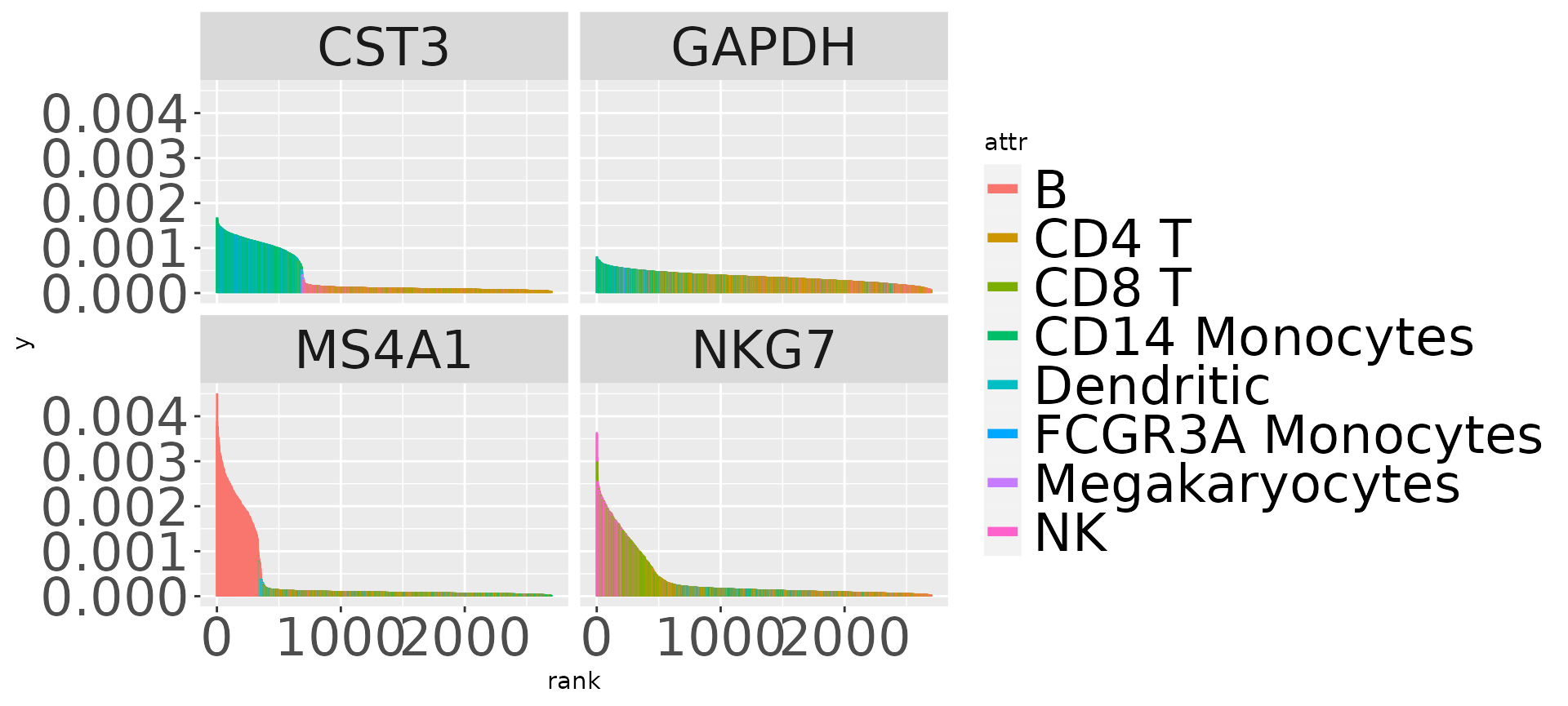
Figure 2d: barcodes
We’ll reuse the pp representation of the 3k PBMC data computed above to illustrate the barcode plotting for multiple genes.
syms = c("CST3", "MS4A1", "NKG7", "GAPDH")
cp = get_3k_cell_emb()
gp = get_3k_gene_emb()
ans = simba_barcode_data(symbols = syms, origad = pp,
    clabel="celltype", simbaref=sref, cembpath = cp,
    gembpath = gp)
library(ggplot2)
ggplot(ans, aes(x=rank, xend=rank, y=0, yend=score, colour=attr)) +
  geom_segment() + facet_wrap(~symbol, ncol=2) +
    theme(strip.text=element_text(size=24),
      legend.text=element_text(size=24),
      axis.text=element_text(size=24)) +
guides(colour = guide_legend(override.aes = list(linetype=1, lwd=2)))
Conclusions
This takes care of the bulk of Figure 2 of the initial SIMBA paper. Data for 2e can be obtained from
Simba4Bioc:::compare_entities(sref, cemb, gemb)Additional vignettes in production will explore multiomic applications.