biocXqtl: flexible molecular QTL assessment

Introduction

eQTL analysis generally involves large data volumes of genotype calls. No standard representation for genotypes has emerged, though VCFs and plink2 files are frequently encountered.

In this package we provide a flexible approach to estimating associations between genotype and molecular phenotypes such as gene expression or DNA methylation. We will use the RangedSummarizedExperiment structure as the primary element for structuring the inputs to association test procedures.

Working with variants from VCF

Thanks to the AWS Open Data project, tabix-indexed VCFs for genotyped lymphoblastoid cell lines from the 1000 genomes project are available. Data from the Multi-Ancestry analysis of Gene Expression are available via Zenodo or Dropbox. In our experience the Dropbox link is more performant.

We have acquired the “DESeq2” gene quantifications from the MAGE archive, and a selection of release genotypes from the associated cell lines.

Data on expression and genotype

The expression data:

library(biocXqtl)

## Warning: package 'GenomicRanges' was built under R version 4.5.2

## Warning: replacing previous import 'BiocGenerics::type' by 'arrow::type' when
## loading 'biocXqtl'

data(mageSE_19)

Genotype data:

dv = demo_vcf()
h = VariantAnnotation::scanVcfHeader(dv)
head(samples(h))

## [1] "HG00096" "HG00100" "HG00105" "HG00108" "HG00110" "HG00113"

length(intersect(samples(h), colnames(mageSE_19)))

## [1] 731

Building an XqtlExperiment

We will focus on SNVs but the genotype information has other types of variants.

Bind the minor allele counts to the expression data:

mins  = minorAlleleCounts(demo_vcf(), GRanges("19:1-50000000"))
mxx = XqtlExperiment(mageSE_19, mins)
colData(mxx) = NULL

The last command above allows us to compute crude measures of association. If we populate colData with covariate information, test procedures in the package will incorporate it.

Creating association statistics with visualizations

The following step uses C++ modules to compute association tests for all genotypes and all gene expression measures in mageSE_19.

sds = rowSds(assay(mxx), na.rm=TRUE)
qq = quantile(sds, .95)
ok = which(sds > qq)
system.time(zzz <- bind_Zs(mxx[ok,]))

## some variants have MAF > 0.5

##    user  system elapsed 
##  98.469  38.866  36.456

Here’s a helper function to visualize one association.

onebox = function(xse, mfeat="ENSG00000174837", vnt="rs4897932", title) {
if (missing(title)) title=""
boxplot(split(as.numeric(assay(xse[mfeat,])),
   as.numeric(data.matrix(mcols(getCalls(xse)[vnt,])))),
   ylab=mfeat, xlab=vnt, main=title)
}
onebox(mxx[ok,], title="MAGE eQTL")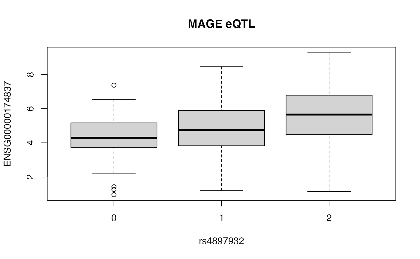

We can also visualize interactively:

viz_stats(zzz, midchop=5)

Covariate adjustment

First we reanalyze with adjustment for continental group.

data(mageSE_19)
sds = rowSds(assay(mageSE_19), na.rm=TRUE)
qq = quantile(sds, .9)
ok = which(sds > qq)
cd = colData(mageSE_19)
mins  = minorAlleleCounts(demo_vcf(), GRanges("19:1-3000000"))
mxx = XqtlExperiment(mageSE_19[ok,], mins)
print(mxx)

## class: XqtlExperiment 
## dim: 138 731 
## metadata(0):
## assays(1): logcounts
## rownames(138): ENSG00000141934 ENSG00000099812 ... ENSG00000196867
##   ENSG00000268107
## rowData names(6): gene_id gene_name ... symbol entrezid
## colnames(731): HG00096 HG00100 ... NA21129 NA21130
## colData names(13): SRA_accession internal_libraryID ...
##   RNAQubitTotalAmount_ng RIN
##   9594 genotype calls present.
##   use getCalls() to see them with addresses.

colData(mxx)=NULL
rowRanges(mxx) = rowRanges(mxx)[,1:6]
mxx$continent = cd$continentalGroup
system.time(zzz <- bind_Zs(mxx))

## some variants have MAF > 0.5

##    user  system elapsed 
##   7.995   1.025   1.578

viz_stats(zzz, midchop=5)

Then we add sex as well.

data(mageSE_19)
sds = rowSds(assay(mageSE_19), na.rm=TRUE)
qq = quantile(sds, .9)
ok = which(sds > qq)
cd = colData(mageSE_19)
mins  = minorAlleleCounts(demo_vcf(), GRanges("19:1-3000000"))
mxx = XqtlExperiment(mageSE_19[ok,], mins)
mxx$continent = cd$continentalGroup
mxx$sex = cd$sex
system.time(zzz <- bind_Zs(mxx))

## some variants have MAF > 0.5

##    user  system elapsed 
##  25.229   1.374   3.859

viz_stats(zzz, midchop=7)