gwaslake: exploring the MRC GWAS API and data/software ecosystem with Bioconductor
Vincent J. Carey, stvjc at channing.harvard.edu
August 09, 2022
Source:vignettes/gwaslake.Rmd
gwaslake.RmdIntroduction
We are indebted to the MRC Integrative Epidemiology Unit for producing the infrastructure leading to the following schematic:
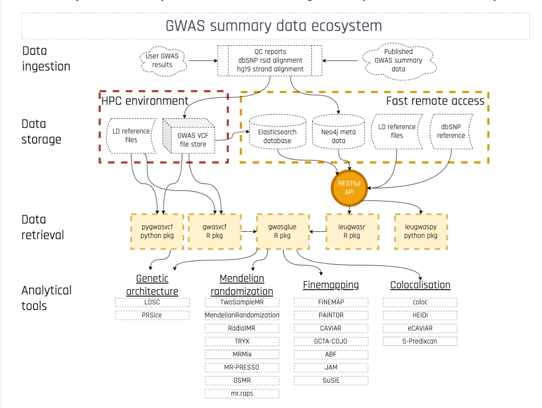
mrc eco
Caveat about software component maintenance
The packages identified in the ecosystem are mostly accessed through github repositories. The interdependencies and idiosyncrasies of using Remotes in DESCRIPTION made it difficult to produce a container image, so I have forked several of the packages identified in the schematic, to tweak the DESCRIPTIONs. I have filed some pull requests but have not heard back. I will try to keep the DESCRIPTION for this workshop package current, minimizing use of forks, and hope individual package maintainers will get in touch.
The API viewed through ieugwasr
We’ll start by listing the functions available in the ieugwasr package.
suppressPackageStartupMessages({
library(gwaslake)
library(plotly)
library(ieugwasr)
library(dplyr)
library(tibble)
library(DT)
library(ontoProc)
})
## API: public: http://gwas-api.mrcieu.ac.uk/
ls("package:ieugwasr")## [1] "%>%" "afl2_chrpos" "afl2_list"
## [4] "afl2_rsid" "api_query" "api_status"
## [7] "associations" "batch_from_id" "batches"
## [10] "check_access_token" "cor" "editcheck"
## [13] "fill_n" "get_access_token" "get_query_content"
## [16] "gwasinfo" "infer_ancestry" "ld_clump"
## [19] "ld_clump_local" "ld_matrix" "ld_matrix_local"
## [22] "ld_reflookup" "legacy_ids" "logging_info"
## [25] "phewas" "revoke_access_token" "select_api"
## [28] "tophits" "variants_chrpos" "variants_gene"
## [31] "variants_rsid" "variants_to_rsid"The pkgdown site for ieugwasr includes a reference listing, visible here.
The gwasinfo command makes an API call to the MRC ecosystem.
gwi = gwasinfo()However, we don’t want to do this too often, so we’ve made a snapshot and keep it in the package.
gwi = gwidf_2021_01_30
as_tibble(gwi)
## # A tibble: 34,513 × 29
## id trait cover…¹ imput…² group…³ year mr author conso…⁴ sex qc_pr…⁵
## <chr> <chr> <chr> <chr> <chr> <int> <int> <chr> <chr> <chr> <chr>
## 1 ieu-b… Alco… whole … HRC public 2019 1 Liu, M GWAS a… Male… "mappe…
## 2 ieu-b… Urin… whole … NA public 2020 1 Zanet… NA Male… NA
## 3 eqtl-… ENSG… NA NA public 2018 1 Vosa U NA Male… NA
## 4 eqtl-… ENSG… NA NA public 2018 1 Vosa U NA Male… NA
## 5 eqtl-… ENSG… NA NA public 2018 1 Vosa U NA Male… NA
## 6 eqtl-… ENSG… NA NA public 2018 1 Vosa U NA Male… NA
## 7 eqtl-… ENSG… NA NA public 2018 1 Vosa U NA Male… NA
## 8 prot-… PDGF… NA NA public 2019 1 Suhre… NA Male… NA
## 9 ubm-a… NET1… NA NA public 2018 1 Ellio… NA Males NA
## 10 prot-… PDZ … NA NA public 2018 1 Sun BB NA Male… NA
## # … with 34,503 more rows, 18 more variables: pmid <int>, population <chr>,
## # sample_size <int>, nsnp <int>, build <chr>, study_design <chr>,
## # covariates <chr>, category <chr>, subcategory <chr>, doi <chr>, note <chr>,
## # priority <int>, unit <chr>, ontology <chr>, sd <dbl>, ncase <int>,
## # ncontrol <int>, batchcode <chr>, and abbreviated variable names ¹coverage,
## # ²imputation_panel, ³group_name, ⁴consortium, ⁵qc_prior_to_upload
## # ℹ Use `print(n = ...)` to see more rows, and `colnames()` to see all variable namesThat’s a huge table. We can get an overview by tabulating the ‘batches’ into which studies have been organized.
Diseases available
A comprehensive view of phenotypes is challenging to assemble. The category field has a relevant value, but we’ll want to explore further.
table(gwi$category)##
## Binary Categorical Ordered Continuous Disease
## 4128 412 4649 140
## Immune system Metabolites NA Risk factor
## 3515 637 20827 205
distab = gwi %>% filter(category=="Disease")
distab %>%
   group_by(trait) %>% summarise(n=n()) %>% arrange(desc(n))
## # A tibble: 82 × 2
## trait n
## <chr> <int>
## 1 Inflammatory bowel disease 7
## 2 Ulcerative colitis 7
## 3 Crohn's disease 6
## 4 Type 2 diabetes 6
## 5 Celiac disease 4
## 6 Coronary heart disease 4
## 7 Multiple sclerosis 4
## 8 Rheumatoid arthritis 4
## 9 Alzheimer's disease 3
## 10 Bipolar disorder 3
## # … with 72 more rows
## # ℹ Use `print(n = ...)` to see more rowsA searchable table will be useful.
datatable(as.data.frame(distab))A visual survey displaying study sizes for selected outcomes
The survey_gwas function plots number of cases versus number of controls for all studies in which the phrases argument matches the trait field, using grep. With plotly, we get an interactive graphic with additional data displayed on hover.
ggplotly(survey_gwas(phrases=c("asthma", "asthmatic")))The survey_app function returns a display like the above, and an interactive table of ‘top hits’.
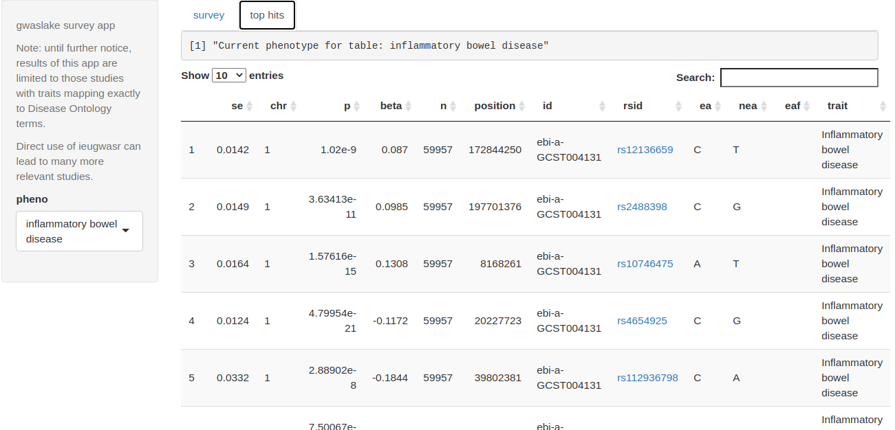
top hits
GWAS hits and their annotation
The pkgdown document on ieugwasr is highly informative. We work through some examples here to verify functionality of our container.
First, by using the searchable table above, we can obtain the study id for “Asthma”: ieu-a-44. We can then obtain the top “hits” for this trait (a p-value threshold can be specified; default is 5e-8).
asthtop = tophits("ieu-a-44")
asthtop
## # A tibble: 8 × 12
## beta n p chr se posit…¹ id rsid ea nea eaf trait
## <dbl> <dbl> <dbl> <chr> <dbl> <int> <chr> <chr> <chr> <chr> <dbl> <chr>
## 1 -0.140 26475 3.52e-12 2 0.0199 1.03e8 ieu-… rs37… A G 0.395 Asth…
## 2 -0.140 26475 1.36e- 8 5 0.0243 1.32e8 ieu-… rs12… C T 0.672 Asth…
## 3 0.148 26475 3.03e-10 5 0.0234 1.10e8 ieu-… rs18… C T 0.741 Asth…
## 4 0.148 26475 1.68e-10 6 0.0241 3.26e7 ieu-… rs17… T C 0.535 Asth…
## 5 -0.171 26475 4.03e-14 9 0.0227 6.21e6 ieu-… rs99… G A 0.787 Asth…
## 6 -0.113 26475 3.93e- 9 15 0.0204 6.74e7 ieu-… rs74… A G 0.503 Asth…
## 7 -0.174 26475 2.77e-18 17 0.0214 3.81e7 ieu-… rs22… C T 0.479 Asth…
## 8 -0.113 26475 1.15e- 8 22 0.0204 3.75e7 ieu-… rs22… A G 0.489 Asth…
## # … with abbreviated variable name ¹positionBasic annotation on these hits can be obtained using either positions or rsids.
asthv = variants_rsid(asthtop$rsid)
datatable(asthv)
PheWAS/eQTL lookup
Let’s follow up our hit in GSDMB with a ‘PheWAS’. The p-value threshold is indicated in documentation to be 0.00001.
A number of the traits are genes, and the findings come from eQTL studies. Let’s see where these genes are located.
##
##  1 10 11 12 14 16 17 18 19  2 20 21 22  3  4  5  6  7  8  9  X
## 20  5  8  4  4  2 21  5  8  8  3  3  3  8 13  6  6  6  8  8  1
So there are ‘trans’ hits for our GSDMB-resident asthma SNP.
Extending the available facilities
Ontological tagging of trait terms
Introduction to Disease Ontology
An ontology is a structured vocabulary, and relationships among terms specified in a directed acyclic graph. Disease Ontology(DO) is an example related to systematic naming of human diseases.
Here is small illustration of the idea.
library(ontoProc)
DO = getDiseaseOnto() # snapshot
## snapshotDate(): 2022-08-09## loading from cache
dem = c("DOID:4", "DOID:7", "DOID:74")
kids = lapply(dem, function(x) DO$children[x][[1]])
onto_plot2(DO, tail(unlist(kids),12))
The formalization of relationships among diseases, as encoded in DO, may be useful in investigations of etiology. The use of formal terms and fixed-length tags will be useful for combining information from independently conducted investigations.
Using Disease Ontology to tag MRC GWAS trait terms
“Traits” studied in the MRC GWAS ecosystem are only infrequently named using formal ontological terms. Simple code to match trait terms with DO terms is
traits = gwidf_2021_01_30$trait
indo = intersect(tolower(traits), tolower(DO$name))
inds = match(indo, tolower(DO$name))
mapped_traits = DO$name[inds]
indo[1:4] # in MRC GWAS
## [1] "agranulocytosis" "radiculopathy" "multiple sclerosis"
## [4] "ovarian dysfunction"
mapped_traits[1:4] # in DO## DOID:12987 DOID:4306 DOID:2377
## "agranulocytosis" "radiculopathy" "multiple sclerosis"
## DOID:1414
## "ovarian dysfunction"
length(mapped_traits)## [1] 195It will be possible to map even more traits once more careful textual analysis is performed on the traits vector. For example, one study uses Diagnoses - main ICD10: K50 Crohn's disease [regional enteritis] to name its trait. The code given above will not find this.
Manhattan plots
The associations function of ieugwasr produces a filtered set of hits for a given region in a given study. The manhattanPlot function of gwaslake simplifies this to some extent, and provides a visualization. One can specify a gene symbol and a flanking radius in base pairs, but one still needs to know the ieugwasr id of the study of interest.
manhattanPlot(studyID="ubm-a-524", symbol = "BCAN", radius=500000)## # A tibble: 6 × 12
## chr p beta posit…¹ n se id rsid ea nea eaf trait
## <chr> <dbl> <dbl> <int> <dbl> <dbl> <chr> <chr> <chr> <chr> <dbl> <chr>
## 1 1 0.794 0.0041 1.56e8 7916 0.0165 ubm-… rs11… T G 0.654 IDP …
## 2 1 0.692 0.0199 1.56e8 7916 0.0508 ubm-… rs12… A G 0.0244 IDP …
## 3 1 0.692 0.0078 1.56e8 7916 0.0197 ubm-… rs72… T C 0.199 IDP …
## 4 1 0.447 0.0125 1.56e8 7916 0.0163 ubm-… rs72… T G 0.350 IDP …
## 5 1 0.501 -0.081 1.56e8 7916 0.120 ubm-… rs57… A G 0.00500 IDP …
## 6 1 0.302 0.0167 1.56e8 7916 0.0161 ubm-… rs46… T C 0.362 IDP …
## # … with abbreviated variable name ¹position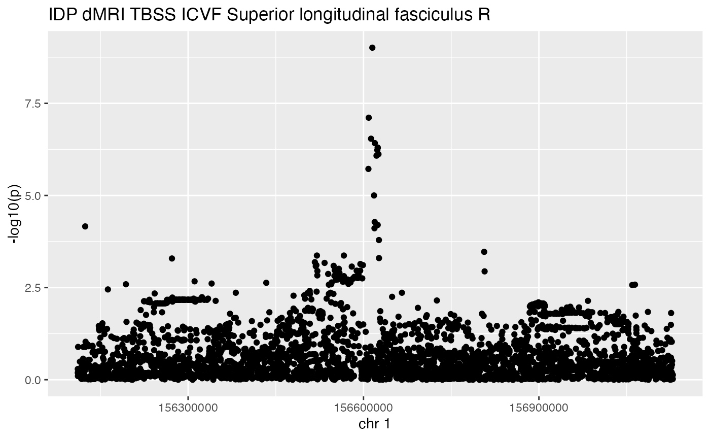
As the tagging of phenotypes improves, this facility will evolve to permit more flexible selection of studies and loci to retrieve and visualize.