B1 Acquiring and exploring 3202 1KG genotypes from chr17 with T2T reference

Objectives

This package demonstrates the use of genotypes obtained via calls against the T2T reference genome. Our objectives are:

acquire and make the genotypes accessible to R/Bioconductor
bind relevant sample-level metadata to the resource
acquire associated RNA-seq assay outputs for a subset of the genotyped samples
perform a series of GWAS to identify expression-based quantitative trait loci (eQTL)

Acquiring 3202 human genotypes called against the T2T reference

The cloud resource; environment variable setting

We have made a large resource available in the hail.is MatrixTable format. This can be retrieved without egress charges using the code in this vignette. A convenient approach uses rclone, as described in the appendix. The zipped MatrixTable folders are at

https://mghp.osn.xsede.org/bir190004-bucket01/Bioc1KGt2t/t17.zip

This 42GB file should be unzipped in a folder to which the environment variable HAIL_T2T_CHR17 will point.

Initial checks of the resource

Ensure that Sys.getenv("HAIL_T2T_CHR17") returns the location of the unzipped MatrixTable resource.

library(BiocT2T)
library(BiocHail)
hl = hail_init()

# NB the following two commands are now encapsulated in the rg_update function
nn <- hl$get_reference('GRCh38')
nn <- nn$read(system.file("json/t2tAnVIL.json", package="BiocHail"))
# updates the hail reference genome
bigloc = Sys.getenv("HAIL_T2T_CHR17")
if (nchar(bigloc)>0) {
  mt17 <- hl$read_matrix_table(Sys.getenv("HAIL_T2T_CHR17"))
  mt17$count()
}

## [[1]]
## [1] 3824434
## 
## [[2]]
## [1] 3202

Population stratification assessment via PCA

PCs in R matrices

The following computation takes close to 30 minutes with 64 cores. We saved the loadings in pc_990kloci.

pcastuff = hl$hwe_normalized_pca(mt17$sample_rows(.25)$GT)

data(pc_990kloci)
pc_990kloci[1:3,1:4]

##                PC1         PC2         PC3          PC4
## HG00096 0.08571635 -0.09670515 -0.04432893  0.032206907
## HG00097 0.07130168 -0.06820003 -0.01072185  0.004602563
## HG00099 0.06578964 -0.08644191 -0.01452058 -0.010706626

PCA has also been performed with samples of 3000 and 190000 loci.

Annotation of samples

The populations of origin of the 3202 samples are tabulated in igsr_pops.

data(igsr_pops)
table(igsr_pops$`Superpopulation code`)

## 
##     AFR AMR EAS EUR SAS 
## 183  10   4   5   5   5

igsr_pops |> dplyr::filter(`Superpopulation code` %in% c("AFR", "SAS")) |> 
    dplyr::select(`Superpopulation name`, `Population code`, `Population name`) |>
    dplyr::arrange(desc(`Superpopulation name`))

##    Superpopulation name Population code     Population name
## 1  South Asian Ancestry             BEB             Bengali
## 2  South Asian Ancestry             PJL             Punjabi
## 3  South Asian Ancestry             GIH            Gujarati
## 4  South Asian Ancestry             STU               Tamil
## 5  South Asian Ancestry             ITU              Telugu
## 6      African Ancestry             ACB   African Caribbean
## 7      African Ancestry             GWW       Gambian Wolof
## 8      African Ancestry             ASW African Ancestry SW
## 9      African Ancestry             YRI              Yoruba
## 10     African Ancestry             GWD    Gambian Mandinka
## 11     African Ancestry             MSL               Mende
## 12     African Ancestry             ESN                Esan
## 13     African Ancestry             LWK               Luhya
## 14     African Ancestry             GWF        Gambian Fula
## 15     African Ancestry             GWJ        Gambian Jola

Latitude and longitude are also available for the population centers from which samples were collected.

Visualizing genetic variation

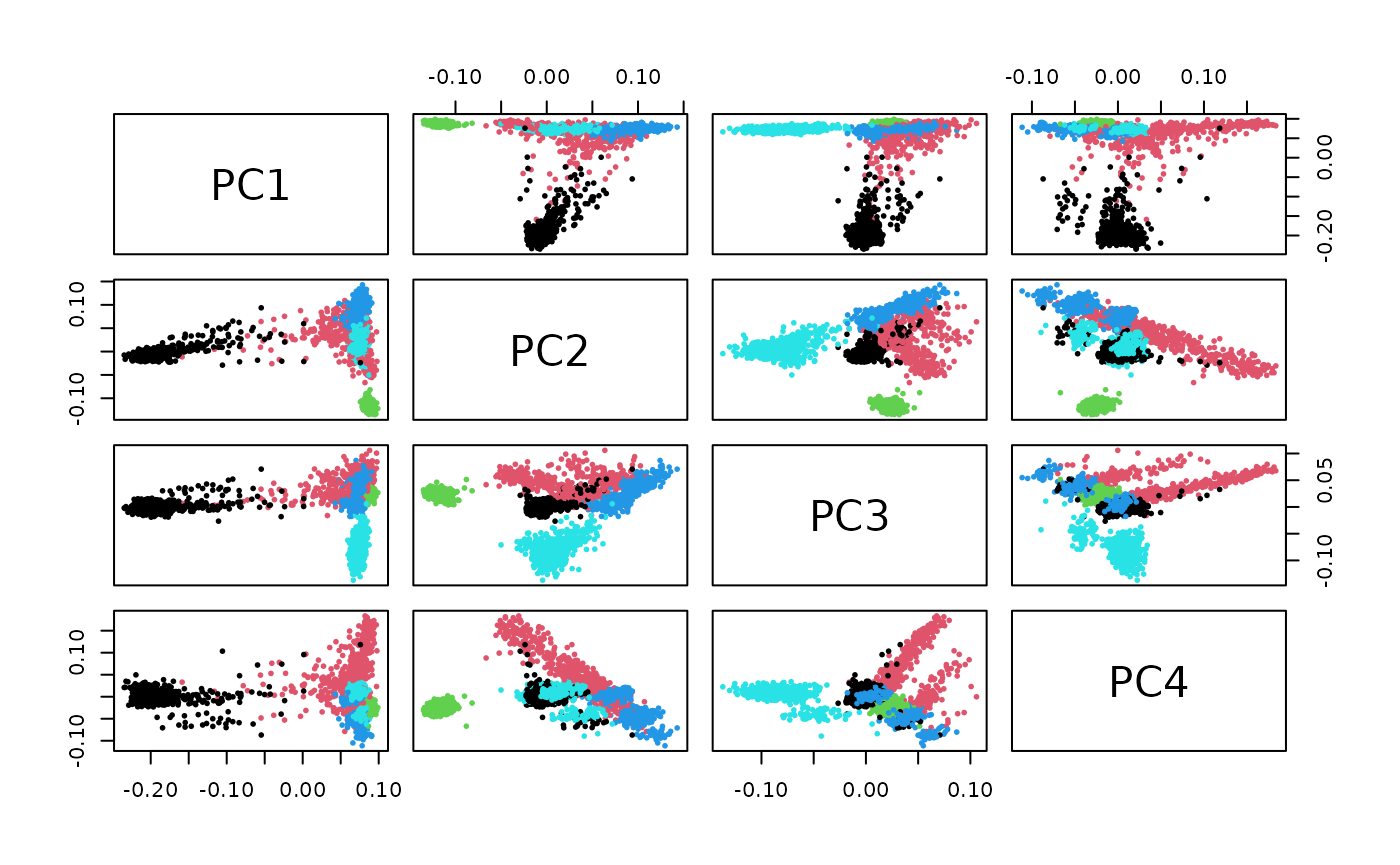
We have several approaches to static visualization of PCs.

A pairs plot for selected PCs for superpopulation visualization based on 190000 loci can be quickly produced.

data(pc_190kloci)
strat2d(pc_190kloci, 1:4, superOnly=TRUE)

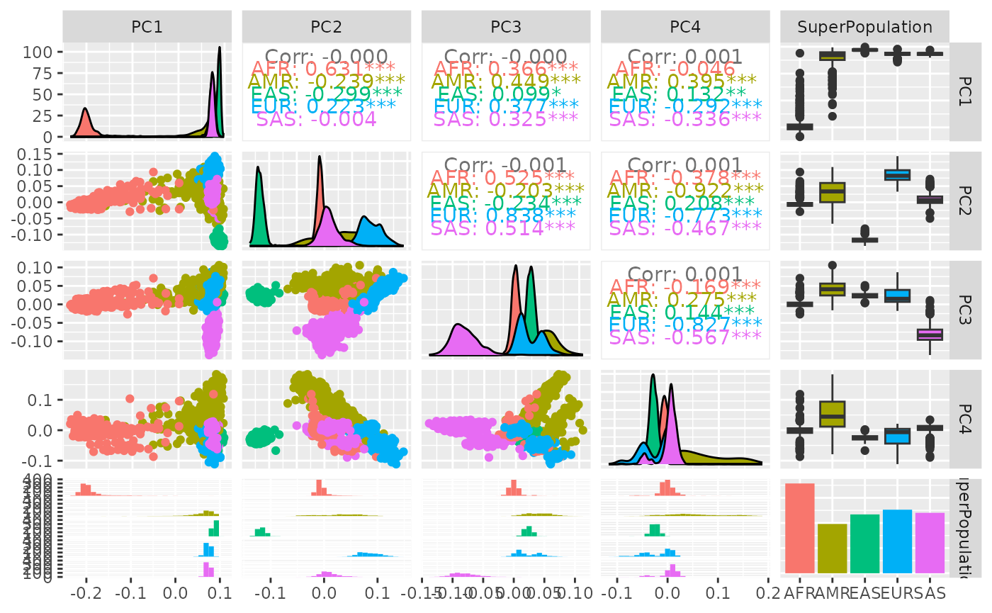
A more carefully annotated view is produced using GGally::ggpairs:

strat2d(pc_190kloci, 1:4, superOnly=TRUE, GGally=TRUE)

Interactive visualization

The stratapp function facilitates simultaneous investigations of

subpopulations within a population
different levels of resolution of genetic detail (size of SNP sample)
specific PCs to use for discrimination

Appendix: Using rclone with docker to get the chr17 data

It can be painful to install and configure rclone. We use a docker container. Let RC_DATADIR be an environment variable evaluating to an available folder.

Also, place the text file with contents

[osn]
type = s3
provider = AWS
endpoint = https://mghp.osn.xsede.org
acl = public
no_check_bucket = true

in a file rclone.conf in a folder pointed to by the environment variable RC_CONFDIR.

Then the following

docker run -v $RC_DATADIR:/data -v $RC_CONFDIR:/config/rclone -t rclone/rclone:latest ls osn:/bir190004-bucket01/Bioc1KGt2t

will list the files with 1KG samples genotyped against the T2T reference.

Use the rclone copyto command to obtain a local copy of the zip file t17.zip in the folder pointed to by $RC_DATADIR:

docker run -v $RC_DATADIR:/data -v $RC_CONFDIR:/config/rclone -t rclone/rclone:latest copyto osn:/bir190004-bucket01/Bioc1KGt2t/t17.zip ./t17.zip

This file should be unzipped in a folder to which the environment variable HAIL_T2T_CHR17 will point.

Vincent J. Carey, stvjc at channing.harvard.edu

April 04, 2023