ontoProc2 -- leveraging semantic SQL for ontology analysis in Bioconductor
Vincent J. Carey, stvjc at channing.harvard.edu
July 13, 2026
Source:vignettes/ontoProc2.Rmd
ontoProc2.RmdIntroduction
The ontoProc2 package has two aims:
- to give convenient access to the ontologies that are transformed to “semantic SQL” in the INCAtools semantic SQL project;
- to simplify operations that have been available in ontoProc, which will be deprecated in 2027.
This package is a “second generation” approach to ontology management and processing for Bioconductor. The ontoProc package was introduced in 2018 and had a number of experimental approaches to interface design and content caching. This package streamlines the identification and management of diverse ontologies by specifically leveraging semantic SQL concepts.
Specifically, the call ontoProc::getOnto('cellOnto')
would produce an ontologyIndex instance. To work with Cell
Ontology with ontoProc2, use semsql_connect(ontology="cl").
The abbreviated notation for ontologies follows that of the Open
Biological and Biomedical Ontologies (OBO) Foundry.
Installation
Prior to the release of Bioconductor 3.24, use
BiocManager::install("vjcitn/ontoProc2").
For Bioconductor 3.24 and subsequent versions, use
BiocManager::install("ontoProc2").
Acquiring ontologies
Make a connection
The best way to work with an ontology in this system is to use
semsql_connect. The ontology argument will be
a short string that the INCAtools project uses as part of the filename
for the ontology. For Gene Ontology, the string is “go”.
library(ontoProc2)
goss <- semsql_connect(ontology = "go")
goss
## <SemsqlConn> prefix: GO | labeled terms: 88,849Make a report
The report method provides details.
report(goss)##
## ============================================================
## SemsqlConn Object
## ============================================================
##
## Connection Details:
## ----------------------------------------
## Database path: /home/runner/.cache/R/BiocFileCache/19c72ffbcde9_go.db
## Ontology prefix: GO
## Status: ✓ Connected
##
## Database Statistics:
## ----------------------------------------
## Labeled terms: 88,849
## Direct edges: 213,852
## Entailed edges: 9,314,992
## Definitions: 55,240
##
## Terms by Prefix (top 5):
## ----------------------------------------
## GO: 48,291
## CHEBI: 24,009
## _: 7,910
## UBERON: 4,783
## CL: 1,307
##
## Key Tables Available:
## ----------------------------------------
## ✓ rdfs_label_statement
## ✓ has_text_definition_statement
## ✓ edge
## ✓ entailed_edge
## ✓ rdfs_subclass_of_statement
## ✓ owl_some_values_from
## ✓ has_oio_synonym_statement
##
## ============================================================
## Use methods like search_labels(), get_ancestors(), etc.
## Run ?SemsqlConn for documentation.
## ============================================================Probe the back end
The back end is SQLite. We can enumerate the tables available:
##
## Attaching package: 'dplyr'
## The following objects are masked from 'package:stats':
##
## filter, lag## The following objects are masked from 'package:base':
##
## intersect, setdiff, setequal, union
library(DBI)
allt <- dbListTables(goss@con)
length(allt)
## [1] 100
head(allt)## [1] "all_problems" "annotation_property_node"
## [3] "anonymous_class_expression" "anonymous_expression"
## [5] "anonymous_individual_expression" "anonymous_property_expression"Use tidy methods
Individual tables are readily accessible.
## # A query:  ?? x 8
## # Database: sqlite 3.53.3 [/home/runner/.cache/R/BiocFileCache/19c72ffbcde9_go.db]
##    stanza                 subject predicate object value datatype language graph
##    <chr>                  <chr>   <chr>     <chr>  <chr> <chr>    <chr>    <chr>
##  1 obo:go/extensions/go-… obo:go… owl:vers… NA     2026… NA       NA       NA
##  2 obo:go/extensions/go-… obo:go… oio:hasO… NA     1.2   NA       NA       NA
##  3 obo:go/extensions/go-… obo:go… oio:defa… NA     gene… NA       NA       NA
##  4 obo:go/extensions/go-… obo:go… dcterms:… cc:by… NA    NA       NA       NA
##  5 obo:go/extensions/go-… obo:go… dce:title NA     Gene… NA       NA       NA
##  6 obo:go/extensions/go-… obo:go… dce:desc… NA     The … NA       NA       NA
##  7 obo:go/extensions/go-… obo:go… IAO:0000… GO:00… NA    NA       NA       NA
##  8 obo:go/extensions/go-… obo:go… IAO:0000… GO:00… NA    NA       NA       NA
##  9 obo:go/extensions/go-… obo:go… IAO:0000… GO:00… NA    NA       NA       NA
## 10 obo:go/extensions/go-… obo:go… owl:vers… obo:g… NA    NA       NA       NA
## # ℹ more rows
tbl(goss@con, "statements") |>
  head(20) |>
  as.data.frame() |>
  datatable()
To investigate the ontology, searching through RDF labels is a natural approach.
search_labels(goss, "apoptosis") |>
  head() |>
  datatable()
Additional filtering could be useful here to focus on GO terms. The
_riog... labels have special roles in RDF inference, and
this will be addressed in vignettes to be added in the future.
Let’s improve the query:
search_labels(goss, "apoptosis") |>
  filter(grepl("^GO:", subject)) |>
  head() |>
  datatable()
Clearly it will be valuable to filter away obsolete terms. We will investigate the use of edge tables to accomplish this in a future vignette.
Transformation to ontology_index instances
The ontologyX suite of Daniel Greene and colleagues provides very convenient ontology handling functions. We can transform the SQLite data to this format. We’ll illustrate with cell ontology.
clss <- semsql_connect(ontology = "cl")## Connected to SemanticSQL database: /home/runner/.cache/R/BiocFileCache/19c7a780bc1_cl.db## Primary ontology prefix: CL
cloi <- semsql_to_oi(clss@con)## Warning in ontologyIndex::ontology_index(name = nn, parents = pl): Some parent
## terms not found: BFO:0000002, BFO:0000004, SO:0000704 (15 more)
cloi## Ontology with 18603 terms
##
## Properties:
## id: character
## name: list
## parents: list
## children: list
## ancestors: list
## obsolete: logical
## Roots:
## UBERON:0000105 - life cycle stage
## GO:0008150 - biological_process
## GO:0003674 - molecular_function
## UBERON:0000465 - material anatomical entity
## UBERON:0000466 - immaterial anatomical entity
## GO:0005575 - cellular_component
## PATO:0000001 - quality
## PR:000010543 - myeloperoxidase
## IAO:0000027 - data entity
## PR:000001338 - complement receptor type 2
## ... 876 moreA convenience function assists with visualizations:
onto_plot2(cloi, c("CL:0000624", "CL:0000492", "CL:0000793", "CL:0000803"))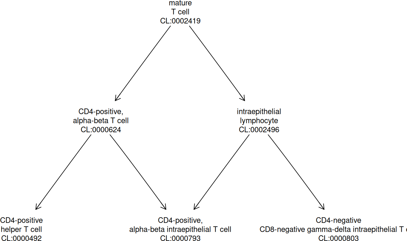
Background
The S7 class design in this package was initiated by a request to Anthropic Claude to use S7 in establishing code that mirrors the tasks accomplished in the INCAtools jupyter notebook.
Searching in label text
The code of search_labels is:
## <S7_method> method(search_labels, ontoProc2::SemsqlConn)
## function (x, pattern, limit = 20L)
## {
##     dbGetQuery(x@con, "SELECT subject, value AS label FROM rdfs_label_statement\n      WHERE value LIKE ? LIMIT ?",
##         param = list(paste0("%", pattern, "%"), as.integer(limit)))
## }
## <environment: namespace:ontoProc2>
Exploring concept properties with ‘edge tables’
The INCAtools notebook discusses the fact that
rdfs_label_statement is a SQLite table “view”.
The notebook indicates that a SPARQL query on an RDF store for the following computation would be “quite hard”. We want to find all the “edges” leading from “enteric neuron”, which would constitute the set of subject-predicate-object statements about this cell type with “enteric neuron” as subject.
In this code we use the concept of a “CURIE” (Compact Uniform Resource Identifier): a fixed length numerical identifier with a prefix indicating the source ontology in which the ontologic concept is based.
if (!is_connected(clss)) clss <- reconnect(clss)
entcurie <- search_labels(clss, "enteric neuron") |>
  filter(grepl("^CL", subject)) |>
  dplyr::select(subject) |>
  unlist()
entcurie
## subject
## "CL:0007011"
get_direct_edges(clss, entcurie)## subject subject_label predicate predicate_label object
## 1 CL:0007011 enteric neuron BFO:0000050 part of UBERON:0002005
## 2 CL:0007011 enteric neuron BFO:0000050 part of UBERON:0002005
## 3 CL:0007011 enteric neuron RO:0002100 has soma location UBERON:0002005
## 4 CL:0007011 enteric neuron RO:0002100 has soma location UBERON:0002005
## 5 CL:0007011 enteric neuron RO:0002202 develops from CL:0002607
## 6 CL:0007011 enteric neuron rdfs:subClassOf <NA> CL:0000029
## 7 CL:0007011 enteric neuron rdfs:subClassOf <NA> CL:0000107
## object_label
## 1 enteric nervous system
## 2 enteric nervous system
## 3 enteric nervous system
## 4 enteric nervous system
## 5 migratory enteric neural crest cell
## 6 neural crest derived neuron
## 7 autonomic neuronHere the underlying code is performing a join:
method(get_direct_edges, SemsqlConn)## <S7_method> method(get_direct_edges, ontoProc2::SemsqlConn)
## function (x, term_id, direction = c("outgoing", "incoming", "both"))
## {
## direction = match.arg(direction)
## query.init <- "SELECT\n e.subject,\n sl.value AS subject_label,\n e.predicate,\n pl.value AS predicate_label,\n e.object,\n ol.value AS object_label\n FROM edge e\n LEFT JOIN rdfs_label_statement sl ON e.subject = sl.subject\n LEFT JOIN rdfs_label_statement pl ON e.predicate = pl.subject\n LEFT JOIN rdfs_label_statement ol ON e.object = ol.subject\n WHERE"
## if (direction == "outgoing") {
## query.fin <- "e.subject = ?"
## query = paste(query.init, query.fin)
## return(dbGetQuery(x@con, query, param = list(term_id)))
## }
## else if (direction == "incoming") {
## query.fin <- "e.object = ?"
## query = paste(query.init, query.fin)
## return(dbGetQuery(x@con, query, param = list(term_id)))
## }
## else if (direction == "both") {
## query.fin <- "e.subject = ? OR e.object = ?"
## query = paste(query.init, query.fin)
## return(dbGetQuery(x@con, query, param = list(term_id,
## term_id)))
## }
## }
## <environment: namespace:ontoProc2>Generalizing a concept: Ancestors
The notebook mentions that the “entailed edges” table includes all statements that can be inferred from the application of base axioms of the ontology.
get_ancestors(clss, entcurie)## id label predicate
## 1 BFO:0000002 <NA> rdfs:subClassOf
## 2 BFO:0000004 <NA> rdfs:subClassOf
## 3 BFO:0000040 <NA> rdfs:subClassOf
## 4 UBERON:0001062 anatomical entity rdfs:subClassOf
## 5 UBERON:0000061 anatomical structure rdfs:subClassOf
## 6 CL:0000107 autonomic neuron rdfs:subClassOf
## 7 CL:0000000 cell rdfs:subClassOf
## 8 CL:0000211 electrically active cell rdfs:subClassOf
## 9 CL:0000393 electrically responsive cell rdfs:subClassOf
## 10 CL:0000404 electrically signaling cell rdfs:subClassOf
## 12 CL:0000255 eukaryotic cell rdfs:subClassOf
## 13 UBERON:0000465 material anatomical entity rdfs:subClassOf
## 14 CL:0002319 neural cell rdfs:subClassOf
## 15 CL:0000029 neural crest derived neuron rdfs:subClassOf
## 16 CL:0000540 neuron rdfs:subClassOf
## 17 CL:2000032 peripheral nervous system neuron rdfs:subClassOfWorking with multiple ontologies
The INCAtools notebook includes an example of finding all neurons that are part of the forebrain. This involves identifying CURIEs for relations and anatomical structures, thus working with the relational ontology (RO) and UBERON.
ub <- semsql_connect(ontology = "uberon")## Connected to SemanticSQL database: /home/runner/.cache/R/BiocFileCache/1cc458b15eb1_uberon.db## Primary ontology prefix: UBERON
ro <- semsql_connect(ontology = "ro")## Connected to SemanticSQL database: /home/runner/.cache/R/BiocFileCache/1c8960098d46_ro.db## Primary ontology prefix: ROFirst question: What’s the CURIE for “forebrain” in UBERON?
fbcur <- search_labels(ub, "forebrain", limit = 1000) |>
  filter(label == "forebrain") |>
  select(subject) |>
  unlist()
fbcur
## subject
## "UBERON:0001890"Second question: What’s the CURIE for “has soma location” in RO?
loccur <- search_labels(ro, "has soma location") |>
  select(subject) |>
  unlist()
loccur
## subject
## "RO:0002100"What’s the CURIE for “neuron”?
ncur <- search_labels(clss, "neuron", limit = 1000) |>
  filter(label == "neuron") |>
  select(subject) |>
  unlist()
ncur
## subject
## "CL:0000540"Now we use three steps to obtain the solution.
First, enumerate all cell types that are located in forebrain.
clinfb <- tbl(clss@con, "entailed_edge") |>
  filter(predicate == loccur, object == fbcur) |>
  select(subject) |>
  collect() |>
  unlist()
length(clinfb)
## [1] 186Second, filter these to those identified as ‘subclassOf’ “neuron”.
clisneur <- tbl(clss@con, "entailed_edge") |>
  filter(predicate == "rdfs:subClassOf", object == ncur) |>
  filter(subject %in% clinfb) |>
  select(subject) |>
  collect() |>
  unlist()
length(clisneur)
## [1] 186Finally, get the labels.
Session information
## R version 4.6.1 (2026-06-24)
## Platform: x86_64-pc-linux-gnu
## Running under: Ubuntu 24.04.4 LTS
##
## Matrix products: default
## BLAS:   /usr/lib/x86_64-linux-gnu/openblas-pthread/libblas.so.3
## LAPACK: /usr/lib/x86_64-linux-gnu/openblas-pthread/libopenblasp-r0.3.26.so;  LAPACK version 3.12.0
##
## locale:
##  [1] LC_CTYPE=C.UTF-8       LC_NUMERIC=C           LC_TIME=C.UTF-8
##  [4] LC_COLLATE=C.UTF-8     LC_MONETARY=C.UTF-8    LC_MESSAGES=C.UTF-8
##  [7] LC_PAPER=C.UTF-8       LC_NAME=C              LC_ADDRESS=C
## [10] LC_TELEPHONE=C         LC_MEASUREMENT=C.UTF-8 LC_IDENTIFICATION=C
##
## time zone: UTC
## tzcode source: system (glibc)
##
## attached base packages:
## [1] stats     graphics  grDevices utils     datasets  methods   base
##
## other attached packages:
## [1] S7_0.2.2          DT_0.34.0         DBI_1.3.0         dplyr_1.2.1
## [5] ontoProc2_0.99.28 BiocStyle_2.40.0
##
## loaded via a namespace (and not attached):
##  [1] xfun_0.60           bslib_0.11.0        httr2_1.2.3
##  [4] htmlwidgets_1.6.4   ontologyPlot_1.7    vctrs_0.7.3
##  [7] tools_4.6.1         crosstalk_1.2.2     generics_0.1.4
## [10] stats4_4.6.1        curl_7.1.0          tibble_3.3.1
## [13] RSQLite_3.53.3      blob_1.3.0          pkgconfig_2.0.3
## [16] R.oo_1.27.1         dbplyr_2.6.0        desc_1.4.3
## [19] graph_1.90.0        lifecycle_1.0.5     compiler_4.6.1
## [22] textshaping_1.0.5   codetools_0.2-20    htmltools_0.5.9
## [25] sass_0.4.10         yaml_2.3.12         pillar_1.11.1
## [28] pkgdown_2.2.1       jquerylib_0.1.4     R.utils_2.13.0
## [31] cachem_1.1.0        tidyselect_1.2.1    digest_0.6.39
## [34] purrr_1.2.2         bookdown_0.47       paintmap_1.0
## [37] fastmap_1.2.0       grid_4.6.1          cli_3.6.6
## [40] magrittr_2.0.5      utf8_1.2.6          withr_3.0.3
## [43] filelock_1.0.3      rappdirs_0.3.4      bit64_4.8.2
## [46] rmarkdown_2.31      bit_4.6.0           otel_0.2.0
## [49] ragg_1.5.2          R.methodsS3_1.8.2   memoise_2.0.1
## [52] evaluate_1.0.5      knitr_1.51          BiocFileCache_3.2.0
## [55] rlang_1.3.0         ontologyIndex_2.12  glue_1.8.1
## [58] Rgraphviz_2.56.0    BiocManager_1.30.27 xml2_1.6.0
## [61] BiocGenerics_0.58.1 jsonlite_2.0.0      R6_2.6.1
## [64] systemfonts_1.3.2   fs_2.1.0