scvi-tools CITE-seq tutorial in R, using serialized tutorial components

A CITE-seq example

The purpose of this vignette is to illustrate the feasibility of reflecting the material in the online tutorial for scvi-tools 0.20.0 in Bioconductor. The authors of the tutorial describe it as producing

a joint latent representation of cells, denoised data for both protein and RNA

Additional tasks include

integrat[ing] datasets, and comput[ing] differential expression of RNA and protein

The integration concerns the simultaneous analysis of two datasets from 10x genomcs.

In this vignette we carry out the bulk of the tutorial activities using R and Bioconductor, reaching to scvi-tools python code via basilisk.

Retrieval of PBMC data

The following chunk will acquire (and cache, using BiocFileCache) a preprocessed version of the 10k and 5k combined CITE-seq experiments from the scvi-tools data repository.

library(scviR)
library(ggplot2)
library(reshape2)
adref = getCiteseq5k10kPbmcs()
adref

## AnnData object with n_obs × n_vars = 10849 × 4000
##     obs: 'n_genes', 'percent_mito', 'n_counts', 'batch', '_scvi_labels', '_scvi_batch'
##     var: 'highly_variable', 'highly_variable_rank', 'means', 'variances', 'variances_norm', 'highly_variable_nbatches'
##     uns: '_scvi_manager_uuid', '_scvi_uuid', 'hvg', 'log1p'
##     obsm: 'protein_expression'
##     layers: 'counts'

Retrieval of fitted VAE

The totalVI variational autoencoder was fit with these data. A fitted version is retrieved and cached using

vae = getCiteseqTutvae()

## INFO     File /home/vincent/TEMP/Rtmp8FzFo7/vae2_ov/model.pt already downloaded 
## INFO     Computing empirical prior initialization for protein background.

This is an instance of an S3 class, python.builtin.object, defined in the reticulate package.

class(vae)

## [1] "scvi.model._totalvi.TOTALVI"               
## [2] "scvi.model.base._rnamixin.RNASeqMixin"     
## [3] "scvi.model.base._vaemixin.VAEMixin"        
## [4] "scvi.model.base._archesmixin.ArchesMixin"  
## [5] "scvi.model.base._base_model.BaseModelClass"
## [6] "scvi.autotune._types.TunableMixin"         
## [7] "python.builtin.object"

Some fields of interest that are directly available from the instance include an indicator of the trained state, the general parameters used to train, and the “anndata” (annotated data) object that includes the input counts and various results of preprocessing:

vae$is_trained

## [1] TRUE

cat(vae$`_model_summary_string`)

## TotalVI Model with the following params: 
## n_latent: 20, gene_dispersion: gene, protein_dispersion: protein, gene_likelihood: nb, latent_distribution: normal

vae$adata

## AnnData object with n_obs × n_vars = 10849 × 4000
##     obs: 'n_genes', 'percent_mito', 'n_counts', 'batch', '_scvi_labels', '_scvi_batch'
##     var: 'highly_variable', 'highly_variable_rank', 'means', 'variances', 'variances_norm', 'highly_variable_nbatches'
##     uns: '_scvi_manager_uuid', '_scvi_uuid', 'hvg', 'log1p'
##     obsm: 'protein_expression'
##     layers: 'counts'

The structure of the VAE is reported using

vae$module

This is quite voluminous and is provided in an appendix.

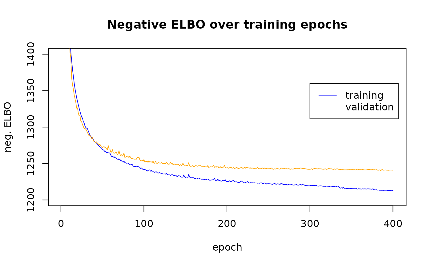
Trace of (negative) ELBO values

The negative “evidence lower bound” (ELBO) is a criterion that is minimized in order to produce a fitted autoencoder. The scvi-tools totalVAE elgorithm creates a nonlinear projection of the inputs to a 20-dimensional latent space, and a decoder that transforms object positions in the latent space to positions in the space of observations that are close to the original input positions.

The negative ELBO values are computed for samples from the training data and for “left out” validation samples. Details on the validation assessment would seem to be part of pytorch lightning. More investigation of scvi-tools code and doc are in order.

h = vae$history
npts = nrow(h$elbo_train)
plot(seq_len(npts), as.numeric(h$elbo_train[[1]]), ylim=c(1200,1400), 
  type="l", col="blue", main="Negative ELBO over training epochs",
  ylab="neg. ELBO", xlab="epoch")
graphics::legend(300, 1360, lty=1, col=c("blue", "orange"), legend=c("training", "validation"))
graphics::lines(seq_len(npts), as.numeric(h$elbo_validation[[1]]), type="l", col="orange")

Normalized quantities

On a CPU, the following can take a long time.

NE = vae$get_normalized_expression(n_samples=25L, 
    return_mean=TRUE, 
    transform_batch=c("PBMC10k", "PBMC5k")
)

We provide the totalVI-based denoised quantities in

denoised = getTotalVINormalized5k10k()
vapply(denoised, dim, integer(2))

##      rna_nmlzd prot_nmlzd
## [1,]     10849      10849
## [2,]      4000         14

Note that these have features as columns, samples (cells) as rows.

utils::head(colnames(denoised$rna_nmlzd))

## [1] "AL645608.8" "HES4"       "ISG15"      "TTLL10"     "TNFRSF18"  
## [6] "TNFRSF4"

utils::head(colnames(denoised$prot_nmlzd))

## [1] "CD3_TotalSeqB"  "CD4_TotalSeqB"  "CD8a_TotalSeqB" "CD14_TotalSeqB"
## [5] "CD15_TotalSeqB" "CD16_TotalSeqB"

UMAP projection of Leiden clustering in the totalVI latent space

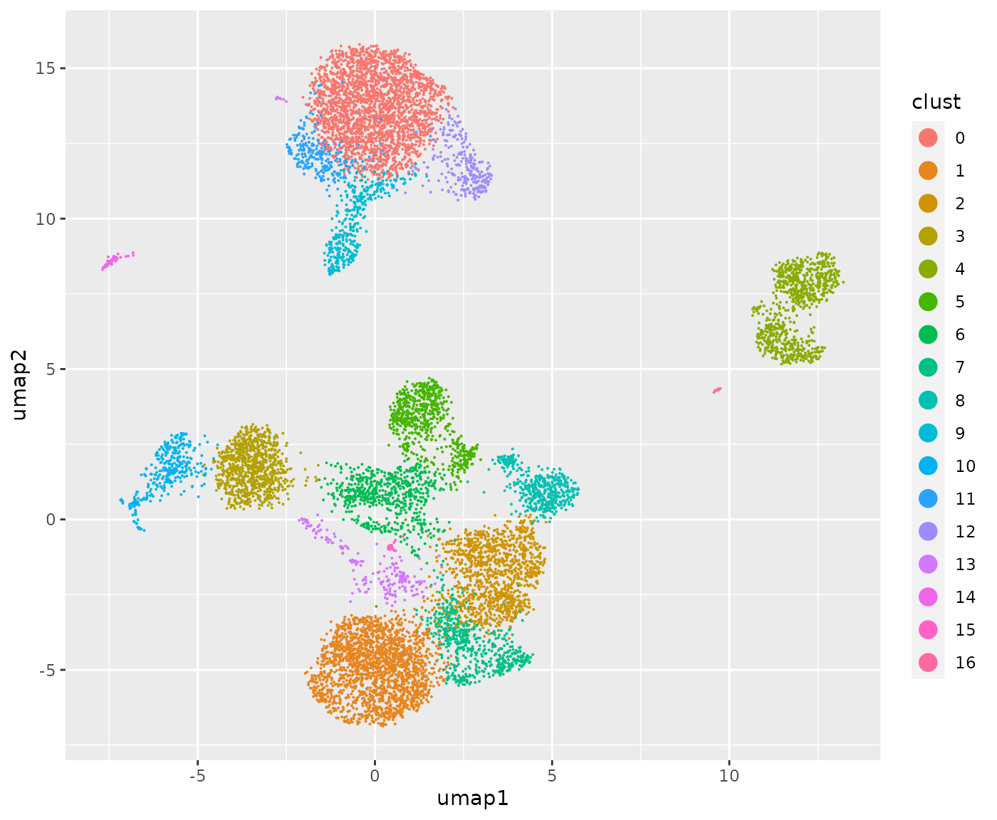
We have stored a fully loaded anndata instance for retrieval to inspect the latent space and clustering produced by the tutorial notebook procedure. The images produced here do not agree exactly with what I see in the colab pages for 0.20.0. The process was run in Jetstream2, not in colab.

full = getTotalVI5k10kAdata()
# class distribution
cllabs = full$obs$leiden_totalVI
blabs = full$obs$batch
table(cllabs)

## cllabs
##    0    1    2    3    4    5    6    7    8    9   10   11   12   13   14   15 
## 2287 1899 1138  866  787  660  637  587  461  375  334  261  260  208   59   19 
##   16 
##   11

um = full$obsm$get("X_umap") 
dd = data.frame(umap1=um[,1], umap2=um[,2], clust=factor(cllabs), batch=blabs)
ggplot(dd, aes(x=umap1, y=umap2, colour=clust)) + geom_point(size=.05) +
   guides(color = guide_legend(override.aes = list(size = 4)))

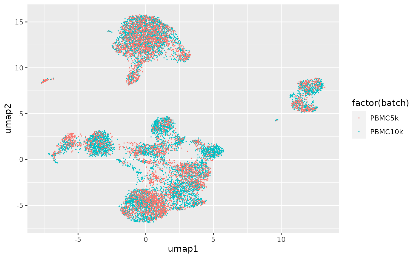
Effectiveness at accommodating the two-batch design is suggested by the mixed representation of the batches in all the Leiden clusters.

ggplot(dd, aes(x=umap1, y=umap2, colour=factor(batch))) + geom_point(size=.05)

Protein abundances in projected clusters

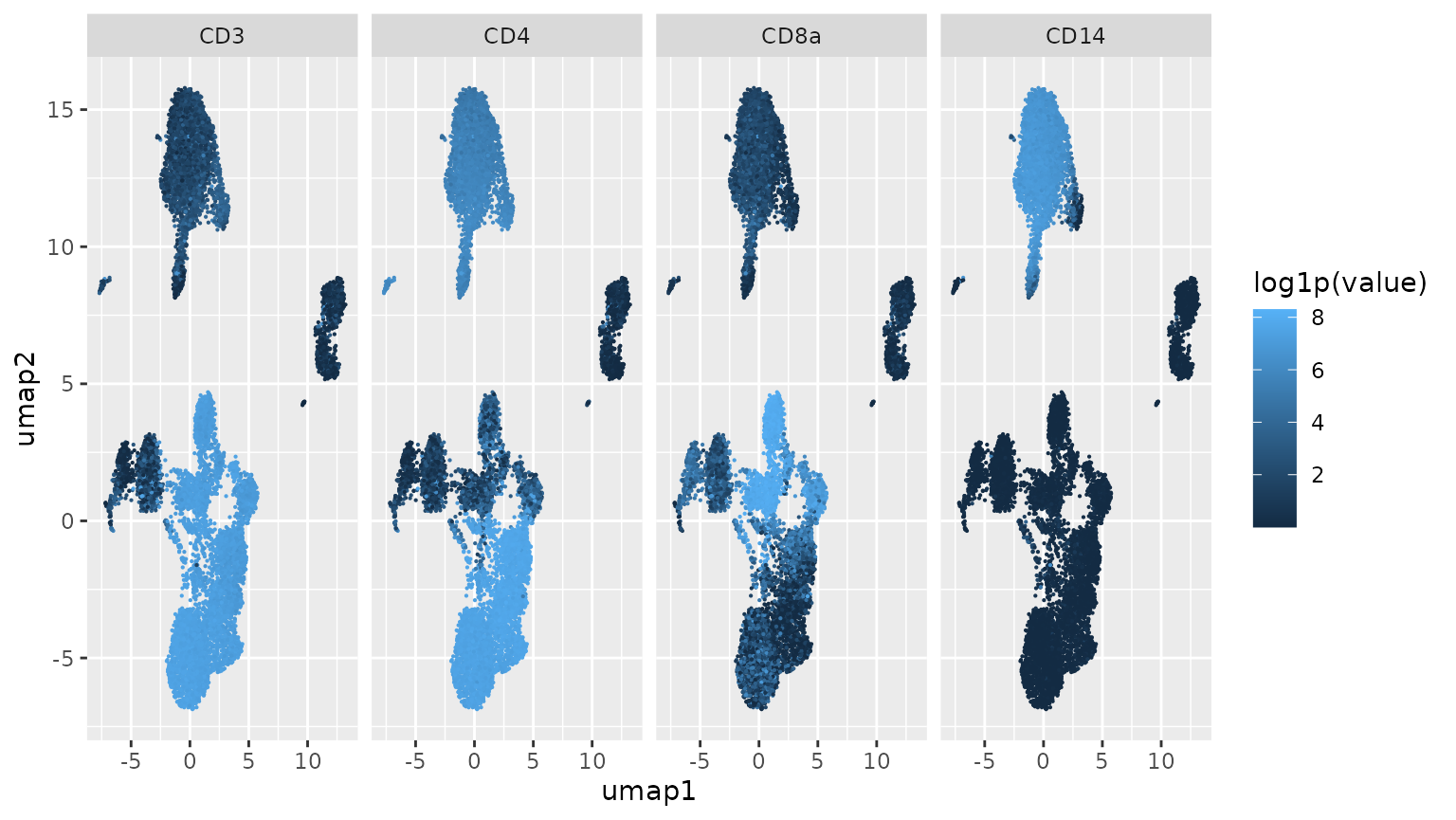
We focus on four of the ADT. Points (cells) in the UMAP projection given above are colored by the estimated abundance of the proteins quantified via (normalized) ADT abundance. Complementary expression of CD4 and CD8a is suggested by the configurations in the middle two panels.

pro4 = denoised$prot_nmlzd[,1:4]
names(pro4) = gsub("_.*", "", names(pro4))
wprot = cbind(dd, pro4)
mm = melt(wprot, id.vars=c("clust", "batch", "umap1", "umap2"))
utils::head(mm,3)

##   clust   batch     umap1    umap2 variable      value
## 1     0 PBMC10k 1.0286884 14.58188      CD3  0.6282051
## 2     0 PBMC10k 0.8443313 15.29502      CD3 11.9159498
## 3     0 PBMC10k 0.8057814 13.96269      CD3  8.9384489

ggplot(mm, aes(x=umap1, y=umap2, colour=log1p(value))) + 
   geom_point(size=.1) + facet_grid(.~variable)

Conclusions

We have shown that all the results of the totalVI application in the tutorial are readily accessible with utilities in scviR. Additional work on details of differential expression are present in the tutorial and can be explored by the interested reader/user.

Appendix: The VAE module