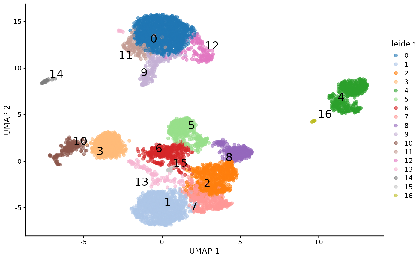
Comparing totalVI and OSCA book CITE-seq analyses
OSCA book authors and Vincent J. Carey, stvjc at channing.harvard.edu
September 26, 2023
Source:vignettes/compch12.Rmd
compch12.RmdOverview
This vignette endeavors to put Bioconductor and scvi-tools together to help understand how different data structures and methods relevant to CITE-seq analysis contribute to interpretation of CITE-seq exeperiments.
The scvi-tools tutorial (for version 0.20.0) analyzes a pair of 10x PBMC CITE-seq experiments (5k and 10k cells). Chapter 12 of the OSCA book analyzes only the 10k dataset.
Technical steps to facilitate comparison
The following subsections are essentially “code-only”. We exhibit steps necessary to assemble a SingleCellExperiment instance with the subset of the totalVI quantifications produced for the cells from the “10k” dataset.
Obtain key data representations
ch12sce = getCh12Sce(clear_cache=FALSE)
ch12sce
## class: SingleCellExperiment
## dim: 33538 7472
## metadata(2): Samples se.averaged
## assays(2): counts logcounts
## rownames(33538): ENSG00000243485 ENSG00000237613 ... ENSG00000277475
## ENSG00000268674
## rowData names(3): ID Symbol Type
## colnames(7472): AAACCCAAGATTGTGA-1 AAACCCACATCGGTTA-1 ...
## TTTGTTGTCGAGTGAG-1 TTTGTTGTCGTTCAGA-1
## colData names(3): Sample Barcode sizeFactor
## reducedDimNames(0):
## mainExpName: Gene Expression
## altExpNames(1): Antibody Capture
fullvi = getTotalVI5k10kAdata()
fullvi
## AnnData object with n_obs × n_vars = 10849 × 4000
## obs: 'n_genes', 'percent_mito', 'n_counts', 'batch', '_scvi_labels', '_scvi_batch', 'leiden_totalVI'
## var: 'highly_variable', 'highly_variable_rank', 'means', 'variances', 'variances_norm', 'highly_variable_nbatches'
## uns: '_scvi_manager_uuid', '_scvi_uuid', 'hvg', 'leiden', 'log1p', 'neighbors', 'umap'
## obsm: 'X_totalVI', 'X_umap', 'denoised_protein', 'protein_expression', 'protein_foreground_prob'
## layers: 'counts', 'denoised_rna'
## obsp: 'connectivities', 'distances'Assemble a SingleCellExperiment with totalVI outputs
Acquire cell identities and batch labels
totvi_cellids = rownames(fullvi$obs)
totvi_batch = fullvi$obs$batch
Acquire quantifications and latent space positions
totvi_latent = fullvi$obsm$get("X_totalVI")
totvi_umap = fullvi$obsm$get("X_umap")
totvi_denoised_rna = fullvi$layers$get("denoised_rna")
totvi_denoised_protein = fullvi$obsm$get("denoised_protein")
totvi_leiden = fullvi$obs$leiden_totalVI
Drop 5k data from all
is5k = which(totvi_batch == "PBMC5k")
totvi_cellids = totvi_cellids[-is5k]
totvi_latent = totvi_latent[-is5k,]
totvi_umap = totvi_umap[-is5k,]
totvi_denoised_rna = totvi_denoised_rna[-is5k,]
totvi_denoised_protein = totvi_denoised_protein[-is5k,]
totvi_leiden = totvi_leiden[-is5k]Find common cell ids
In this section we reduce the cell collections to cells common to the chapter 12 and totalVI datasets.
comm = intersect(totvi_cellids, ch12sce$Barcode)Build the totalVI SingleCellExperiment
# select and order
totvi_latent = totvi_latent[comm,]
totvi_umap = totvi_umap[comm,]
totvi_denoised_rna = totvi_denoised_rna[comm,]
totvi_denoised_protein = totvi_denoised_protein[comm,]
totvi_leiden = totvi_leiden[comm]

# organize the totalVI into SCE with altExp

totsce = SingleCellExperiment(SimpleList(logcounts=t(totvi_denoised_rna))) # FALSE name
rowData(totsce) = S4Vectors::DataFrame(fullvi$var)
rownames(totsce) = rownames(fullvi$var)
rowData(totsce)$Symbol = rownames(totsce)
nn = SingleCellExperiment(SimpleList(logcounts=t(totvi_denoised_protein))) # FALSE name
reducedDims(nn) = list(UMAP=totvi_umap)
altExp(totsce) = nn
altExpNames(totsce) = "denoised_protein"
totsce$leiden = totvi_leiden
altExp(totsce)$leiden = totvi_leiden
altExp(totsce)$ch12.clusters = altExp(ch12sce[,comm])$label

# add average ADT abundance to metadata, for adt_profiles

tot.se.averaged <- sumCountsAcrossCells(altExp(totsce), altExp(totsce)$leiden,
    exprs_values="logcounts", average=TRUE)
rownames(tot.se.averaged) = gsub("_TotalSeqB", "", rownames(tot.se.averaged))
metadata(totsce)$se.averaged = tot.se.averaged
Reduce the chapter 12 dataset to the cells held in common
colnames(ch12sce) = ch12sce$Barcode
ch12sce_matched = ch12sce[, comm]
Key outputs of the chapter 12 analysis
Clustering and projection based on the ADT quantifications
The TSNE projection of the normalized ADT quantifications and the walktrap cluster assignments are produced for the cells common to the two approaches.
## Warning: Removed 1 rows containing missing values (`geom_text_repel()`).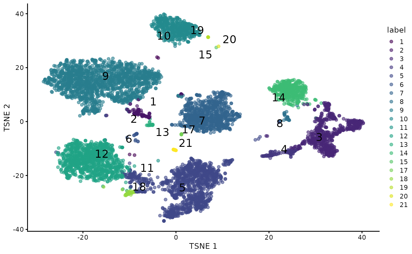
Cluster profiles based on averaging ADT quantities within clusters
This heatmap uses precomputed cluster averages that are lodged in the metadata element of the SingleCellExperiment. Colors represent the log2-fold change from the grand average across all clusters.
adtProfiles(ch12sce_matched)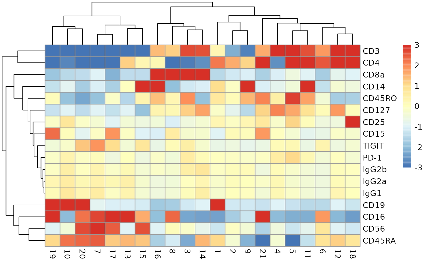
Marker expression patterns in mRNA-based sub-clusters of ADT-based clusters
We enhance the annotation of the list of subclusters retrieved using getCh12AllSce and then drill into mRNA-based subclusters of ADT-based cluster 3 to compare expression levels of three genes.
ch12_allsce = getCh12AllSce()
ch12_allsce = lapply(ch12_allsce, function(x) {
   colnames(x)= x$Barcode;
   cn = colnames(x);
   x = x[,intersect(cn,comm)]; x})
of.interest <- "3"
markers <- c("GZMH", "IL7R", "KLRB1")
plotExpression(ch12_allsce[[of.interest]], x="subcluster",
    features=markers, swap_rownames="Symbol", ncol=3)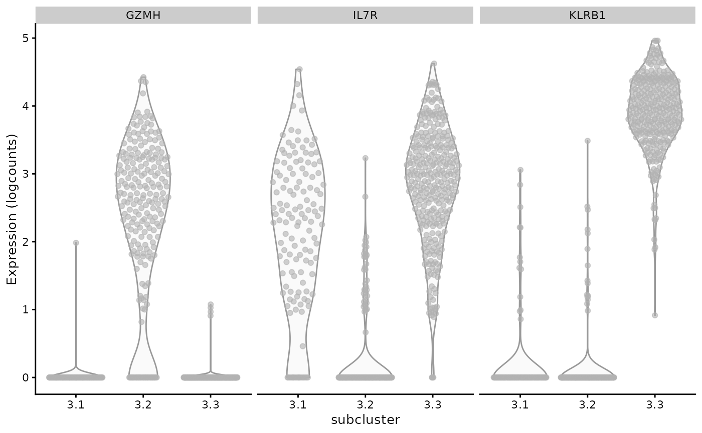
There is a suggestion of a boolean basis for subcluster identity, depending on low or high expression of the selected genes.
Graduated relationships between mRNA and surface protein expression
Following the exploration in OSCA chapter 12, cluster 3 is analyzed for a regression association between expression measures of three genes and the ADT-based abundance of CD127.
plotExpression(ch12_allsce[["3"]], x="CD127", show_smooth=TRUE, show_se=FALSE,
    features=c("IL7R", "TPT1", "KLRB1", "GZMH"), swap_rownames="Symbol")
## `geom_smooth()` using method = 'loess' and formula = 'y ~ x'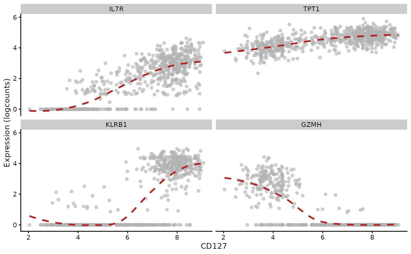
Analogs to the chapter 12 findings, based on totalVI quantifications
Cluster profiles based on average ADT abundance, using denoised protein quantifications
The approach to profiling the ADT abundances used in the totalVI tutorial employs scaling to (0,1).
tav = S4Vectors::metadata(totsce)$se.averaged
ata = assay(tav)
uscale = function(x) (x-min(x))/max(x)
scmat = t(apply(ata,1,uscale))
pheatmap::pheatmap(scmat, cluster_rows=FALSE)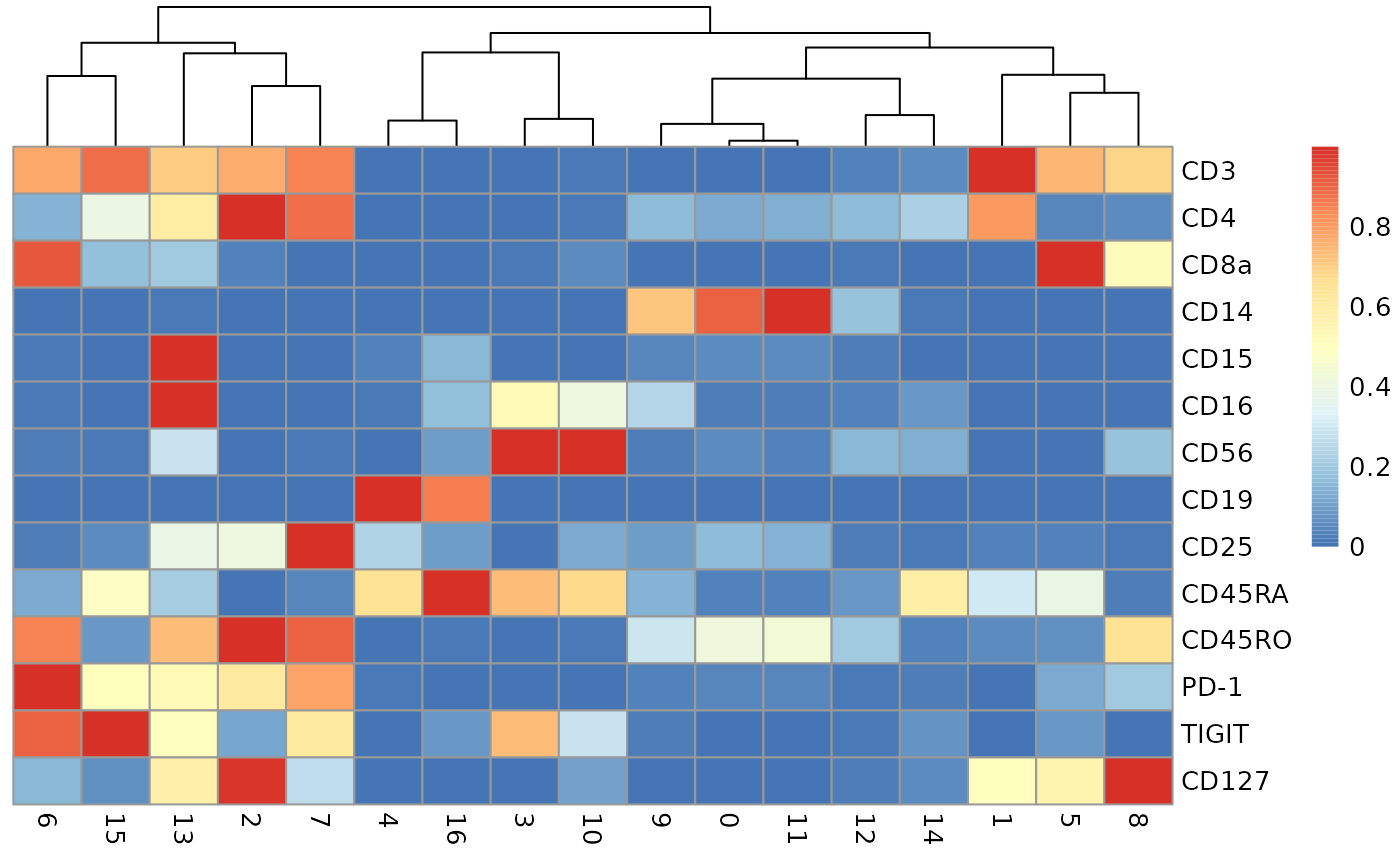
Concordance in ADT-based clustering between OSCA and totalVI
A quick view of the concordance of the two clustering outcomes is
atot = altExp(totsce)
ach12 = altExp(ch12sce_matched)
tt = table(ch12=ach12$label, VI=atot$leiden)
pheatmap::pheatmap(log(tt+1))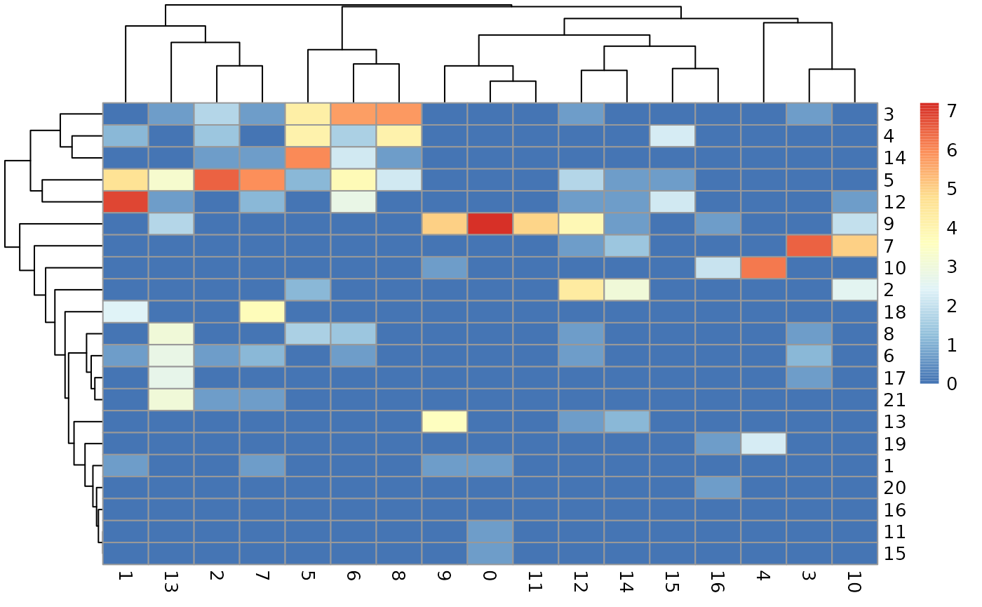
With this we can pick out some clusters with many cells in common:
lit = tt[c("9", "12", "5", "3"), c("0", "1", "2", "8", "6", "5")]
rownames(lit) = sQuote(rownames(lit))
colnames(lit) = sQuote(colnames(lit))
lit
## VI
## ch12 '0' '1' '2' '8' '6' '5'
## '9' 1334 0 0 0 0 0
## '12' 0 993 0 0 15 0
## '5' 0 102 671 8 44 2
## '3' 0 0 5 322 297 67Subcluster assessment for OSCA cluster “3”
Let’s examine the distributions of marker mRNAs in the Leiden totalVI clusters corresponding to OSCA cluster “3”:
tsub = totsce[,which(altExp(totsce)$leiden %in% c("5", "6", "8"))]
markers <- c("GZMH", "IL7R", "KLRB1")
altExp(tsub)$leiden = factor(altExp(tsub)$leiden) # squelch unused levels
tsub$leiden = factor(tsub$leiden) # squelch unused levels
plotExpression(tsub, x="leiden",
    features=markers, swap_rownames="Symbol", ncol=3)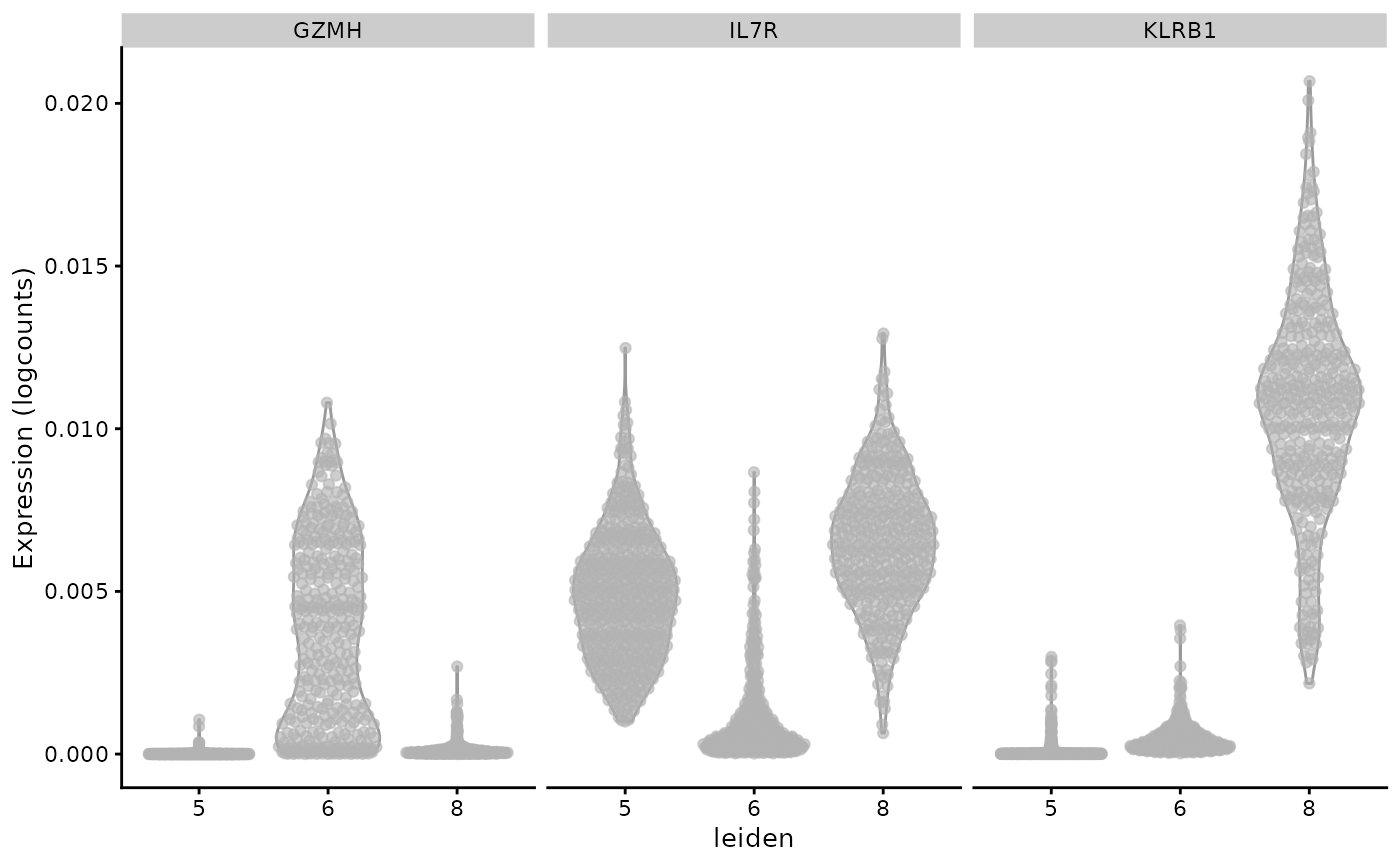
Note that the y axis label is incorrect – we are plotting the denoised expression values from totalVI.
The display seems roughly consistent with the “boolean basis” observed above with the mRNA-based subclustering.
Graduated relationships between ADT and mRNA abundance as measured by totalVI
The same approach is taken as above. We don’t have TPT1 in the 4000 genes retained in the totalVI exercise.
rn = rownames(altExp(tsub))
rn = gsub("_TotalSeqB", "", rn)
rownames(altExp(tsub)) = rn
rowData(altExp(tsub)) = DataFrame(Symbol=rn)
plotExpression(tsub, x="CD127", show_smooth=TRUE, show_se=FALSE,
   features=c("IL7R", "KLRB1", "GZMH"), swap_rownames="Symbol")
## `geom_smooth()` using method = 'gam' and formula = 'y ~ s(x, bs = "cs")'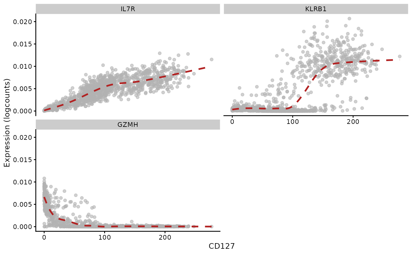
Conclusions
We have shown how rudimentary programming and data organization can be used to make outputs of OSCA and totalVI methods amenable to comparison in the Bioconductor framework.
The scviR package includes a shiny app in the function explore_subcl that should be expanded to facilitate exploration of totalVI subclusters. Much more work remains to be done in the area of exploring
additional approaches to integrative interpretation of ADT and mRNA abundance patterns, such as intersection and concatenation methods in the feature selection materials in OSCA ch. 12
effects of tuning and architecture details for the totalVI VAE
Session information
utils::sessionInfo()## R version 4.3.1 Patched (2023-08-27 r85021)
## Platform: x86_64-pc-linux-gnu (64-bit)
## Running under: Ubuntu 22.04.3 LTS
##
## Matrix products: default
## BLAS: /home/vincent/R-4-3-dist/lib/R/lib/libRblas.so
## LAPACK: /home/vincent/R-4-3-dist/lib/R/lib/libRlapack.so; LAPACK version 3.11.0
##
## locale:
## [1] LC_CTYPE=en_US.UTF-8 LC_NUMERIC=C
## [3] LC_TIME=en_US.UTF-8 LC_COLLATE=en_US.UTF-8
## [5] LC_MONETARY=en_US.UTF-8 LC_MESSAGES=en_US.UTF-8
## [7] LC_PAPER=en_US.UTF-8 LC_NAME=C
## [9] LC_ADDRESS=C LC_TELEPHONE=C
## [11] LC_MEASUREMENT=en_US.UTF-8 LC_IDENTIFICATION=C
##
## time zone: America/New_York
## tzcode source: system (glibc)
##
## attached base packages:
## [1] stats graphics utils stats4 methods base
##
## other attached packages:
## [1] scviR_1.1.1 shiny_1.7.5
## [3] basilisk_1.13.1 scater_1.29.4
## [5] ggplot2_3.4.3 scuttle_1.11.2
## [7] SingleCellExperiment_1.23.0 SummarizedExperiment_1.31.1
## [9] Biobase_2.61.0 GenomicRanges_1.53.1
## [11] GenomeInfoDb_1.37.4 IRanges_2.35.2
## [13] S4Vectors_0.39.1 BiocGenerics_0.47.0
## [15] MatrixGenerics_1.13.1 matrixStats_1.0.0
## [17] BiocStyle_2.29.1
##
## loaded via a namespace (and not attached):
## [1] DBI_1.1.3 bitops_1.0-7
## [3] gridExtra_2.3 rlang_1.1.1
## [5] magrittr_2.0.3 RSQLite_2.3.1
## [7] compiler_4.3.1 mgcv_1.9-0
## [9] dir.expiry_1.9.0 DelayedMatrixStats_1.23.4
## [11] png_0.1-8 systemfonts_1.0.4
## [13] vctrs_0.6.3 stringr_1.5.0
## [15] pkgconfig_2.0.3 crayon_1.5.2
## [17] fastmap_1.1.1 dbplyr_2.3.3
## [19] ellipsis_0.3.2 XVector_0.41.1
## [21] labeling_0.4.3 utf8_1.2.3
## [23] promises_1.2.1 rmarkdown_2.24
## [25] grDevices_4.3.1 ggbeeswarm_0.7.2
## [27] ragg_1.2.5 bit_4.0.5
## [29] purrr_1.0.2 xfun_0.40
## [31] zlibbioc_1.47.0 cachem_1.0.8
## [33] beachmat_2.17.16 jsonlite_1.8.7
## [35] blob_1.2.4 later_1.3.1
## [37] DelayedArray_0.27.10 BiocParallel_1.35.4
## [39] irlba_2.3.5.1 parallel_4.3.1
## [41] R6_2.5.1 RColorBrewer_1.1-3
## [43] bslib_0.5.1 stringi_1.7.12
## [45] limma_3.57.7 reticulate_1.32.0
## [47] jquerylib_0.1.4 Rcpp_1.0.11
## [49] bookdown_0.35 knitr_1.44
## [51] splines_4.3.1 httpuv_1.6.11
## [53] Matrix_1.6-1 tidyselect_1.2.0
## [55] abind_1.4-5 yaml_2.3.7
## [57] viridis_0.6.4 codetools_0.2-19
## [59] curl_5.0.2 lattice_0.21-8
## [61] tibble_3.2.1 basilisk.utils_1.13.3
## [63] withr_2.5.0 evaluate_0.21
## [65] desc_1.4.2 BiocFileCache_2.9.1
## [67] pillar_1.9.0 BiocManager_1.30.22
## [69] filelock_1.0.2 generics_0.1.3
## [71] rprojroot_2.0.3 RCurl_1.98-1.12
## [73] sparseMatrixStats_1.13.4 munsell_0.5.0
## [75] scales_1.2.1 xtable_1.8-4
## [77] glue_1.6.2 pheatmap_1.0.12
## [79] tools_4.3.1 datasets_4.3.1
## [81] BiocNeighbors_1.19.0 ScaledMatrix_1.9.1
## [83] fs_1.6.3 cowplot_1.1.1
## [85] grid_4.3.1 colorspace_2.1-0
## [87] nlme_3.1-163 GenomeInfoDbData_1.2.10
## [89] beeswarm_0.4.0 BiocSingular_1.17.1
## [91] vipor_0.4.5 cli_3.6.1
## [93] rsvd_1.0.5 textshaping_0.3.6
## [95] fansi_1.0.4 S4Arrays_1.1.6
## [97] viridisLite_0.4.2 dplyr_1.1.3
## [99] gtable_0.3.4 sass_0.4.7
## [101] digest_0.6.33 SparseArray_1.1.12
## [103] ggrepel_0.9.3 farver_2.1.1
## [105] memoise_2.0.1 htmltools_0.5.6
## [107] pkgdown_2.0.7 lifecycle_1.0.3
## [109] httr_1.4.7 statmod_1.5.0
## [111] mime_0.12 bit64_4.0.5